

Название-Сеть в Играх 2006год_Язык-Eng
.pdf44 Networking and Online Games: Understanding and Engineering Multiplayer Internet Games
In other words, an IP address represents both the identity of the attached host and the host’s ‘location’ on the network. (This location is topological rather than geographical. It reflects where the host exists within the interconnections of IP networks and service providers that make up the Internet.)
IP addresses are closely related to, but not the same as, Fully Qualified Domain Names (FQDNs, or simply ‘domain names’). Domain names (often imprecisely referred to as Internet addresses) are textual addresses of the form ‘www.gamespy.com’, ‘www.freebsd.org’ or ‘www.bbc.co.uk’. Domain names must be resolved into IP addresses using the Domain Name System (DNS). Endpoint applications typically hide this translation step from the user, and use the resulting numeric IP address to establish communication with the intended destination. (We will discuss the DNS in greater detail later in this chapter.)
4.1.2 Layered Transport Services
Most game developers will utilise IP in conjunction with either the TCP [RFC793] or UDP [RFC768]. TCP and UDP are transport protocols, designed to provide another layer of abstraction on top of the IP layer’s network service. Both TCP and UDP support the concurrent multiplexing of data from multiple applications onto a single stream of IP packets between two IP hosts. TCP additionally provides reliable delivery on top of the IP network’s best effort service.
4.1.2.1 Transmission Control Protocol (TCP)
Early Internet applications – such as email, file transfer protocols and remote console login services – were sensitive to packet loss but relatively insensitive to timeliness (everything sent had to be received, but delays from tens of milliseconds to a few seconds were tolerable). The common end-to-end transport requirements of such applications (reliable ordered transfer of bytes from one endpoint to another) motivated development of TCP.
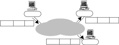
TCP sits immediately above the IP layer within a host (see Figure 4.3), and creates bidirectional paths (sometimes referred to as TCP connections or TCP sessions) between endpoints. An application’s outbound data is broken up and transmitted inside TCP frames, which are themselves carried inside IP packets across the network to the destination. The
|
TCP |
TCP payload |
|
|
TCP layer |
header |
(application data) |
TCP layer |
|
|
|
|||
IP layer |
|
|
IP layer |
|
136.80.1.2 |
Destination Source |
142.8.20.8 |
||
142.8.20.8 136.80.1.2 TCP Frame |
||||
|
|
|||
IP Network
Figure 4.3 TCP runs transparently across the IP network

Basic Internet Architecture |
45 |
|
|
destination host’s TCP layer explicitly acknowledges received TCP frames, enabling the transmitting TCP layer to detect when losses have occurred. Lost TCP frames are retransmitted until acknowledged by the destination, ultimately ensuring that the application’s data is transferred with a high degree of reliability.
TCP uses windowed flow control to regulate how fast it transmits packets through the network. The current window size dictates how many unacknowledged packets may be in transit across the network at any given time. The source grows its window as packets are transmitted successfully, and shrinks its window when packet loss is detected (on the assumption that packets are only lost when the network is briefly overloaded). This regulates the bandwidth consumed by a TCP connection. Flow control and retransmission are handled independently in each direction.
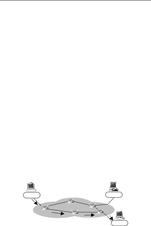
Because TCP may keep retransmitting for many seconds when faced with repeated packet loss, the end application can experience unpredictable variations in latency (Figure 4.4). Thus, TCP is generally not suitable as the transport protocol for real-time messaging during game play of highly interactive networked games.
4.1.2.2 User Datagram Protocol (UDP)
UDP is a much simpler sibling of TCP, providing a connectionless, unreliable, datagramoriented transport service for applications that do not require or desire the overhead of TCP’s service. UDP imposes no flow control on packet transmission, and no packet loss detection or recovery. It is essentially a multiplexing layer sitting directly on top of IP’s best effort service. As such an application using UDP will directly experience the latency, jitter and loss characteristics of the underlying IP network.
4.1.2.3 Multiplexing and Flows
Extending the postal service analogy a little further, while the IP address is analogous to a street address both TCP and UDP add the notion of ports – additional identification analogous to an apartment number or hotel room number. Each TCP or UDP frame carries two 16 bit port numbers to identify the source and destination of their frame within the context of a particular source or destination IP host. This allows multiplexing of different traffic streams between different applications residing on the same source and destination IP endpoints.
|
|
|
|
Application data flow |
|
|
|
|
Applications |
|
|
Applications |
|
||||
|
|
|
|
|||||
|
|
|
|
Losses here cause delays here |
|
|
|
|
|
|
|
|
|
|
|
||
|
|
TCP layer |
TCP layer |
|
|
|||
|
|
|
|
|
|
|
||
IP Network
Figure 4.4 TCP converts IP layer packet loss into application layer delays

46 Networking and Online Games: Understanding and Engineering Multiplayer Internet Games
0 |
|
1 |
|
2 |
3 |
0 1 2 |
3 4 5 6 7 8 |
9 0 1 2 3 4 |
5 6 7 8 9 |
0 1 2 3 4 5 6 |
7 8 9 0 1 |
+-+-+-+-+-+-+-+-+- +-+-+-+-+-+- +-+-+-+-+-+ -+-+-+-+-+-+-+ -+-+-+-+-+
|Version| IHL |Type of Service| Total Length |
+-+-+-+-+-+-+-+-+- +-+-+-+-+-+- +-+-+-+-+-+ -+-+-+-+-+-+-+ -+-+-+-+-+
| Identification |Flags| Fragment Offset |
+-+-+-+-+-+-+-+-+- +-+-+-+-+-+- +-+-+-+-+-+ -+-+-+-+-+-+-+ -+-+-+-+-+ | Time to Live | Protocol | Header Checksum |
+-+-+-+-+-+-+-+-+- +-+-+-+-+-+- +-+-+-+-+-+ -+-+-+-+-+-+-+ -+-+-+-+-+ | Source Address |
+-+-+-+-+-+-+-+-+- +-+-+-+-+-+- +-+-+-+-+-+ -+-+-+-+-+-+-+ -+-+-+-+-+ | Destination Address |
+-+-+-+-+-+-+-+-+- +-+-+-+-+-+- +-+-+-+-+-+ -+-+-+-+-+-+-+ -+-+-+-+-+
| Options | Padding |
+-+-+-+-+-+-+-+-+- +-+-+-+-+-+- +-+-+-+-+-+ -+-+-+-+-+-+-+ -+-+-+-+-+ | Source Port Destination Port |
+-+-+-+-+-+-+-+-+- +-+-+-+-+-+- +-+-+-+-+-+ -+-+-+-+-+-+-+ -+-+-+-+-+
IPv4 header
TCP/UDP ports
Figure 4.5 Header fields of interest in IPv4 packets
IP address and port number combinations are often written in the form ‘ip-address:port’, with a ‘:’ separating the address (either in dotted-quad or fully qualified domain name form) and the numerical port number.
Figure 4.5 shows the key fields of an IPv4 header and the first 32 bits of the TCP or UDP transport header. The protocol field specifies whether the IP packet carries TCP (protocol 6), UDP (protocol 17), or some other type of frame (discussed further in ‘Directory of General Assigned Numbers’ [IANAP]). The source and destination addresses identify a packet’s source and destination host at the IP level.
Taken together, port numbers and IP addresses uniquely identify the source and destination applications that are generating and consuming the traffic. A sequence of packets exchanged between the same TCP or UDP ports on the same two endpoints is often referred to as an application flow (or just flow ). Many applications use ‘well-known’ port numbers, often making it possible to infer the identity of an application from the source or destination port numbers. For example, the Simple Mail Transport Protocol (SMTP) typically uses TCP to port 25 on the mail server host [RFC2821], Quake III Arena servers default to using UDP port 27960, Half-Life 2 servers default to using UDP port 27015 and web servers typically respond to Hypertext Transport Protocol (HTTP) traffic on TCP port 80 [RFC2616].
Note that there are no rules preventing applications from using unconventional ports – we could, for example, just as easily run Quake III Arena on port 27015 and Half-Life 2 on port 27960, so long as everyone knows what is happening.
4.1.3 Unicast, Broadcast and Multicast
Sending a packet to a single destination is known as unicast transmission. Sending a packet to all destinations (within some specified region of the network) is known as broadcast transmission. Broadcasting may be implemented as multiple separate unicast transmissions, but this requires the source to actually know the IP addresses of all intended destinations. Usually the network supports broadcast natively – the source sends a single
Basic Internet Architecture |
47 |
|
|
136.80.1.2 |
142.8.20.8 |
Destination Source Payload
Destination Source 224.50.1.8 136.80.1.2
224.50.1.8 136.80.1.2 Payload
IP Network
Destination |
Source |
Payload |
21.80.1.32 |
224.50.1.8 |
136.80.1.2 |
Figure 4.6 IP multicasting replicates a single packet to (potentially multiple) group members
packet into the network with a specific ‘broadcast’ destination address, and the network itself replicates the packet to all attached hosts within a restricted region.
A little-used alternative is IP multicast [RFC1112]. A source transmits one packet and the network itself delivers identical copies to multiple destinations (known as a multicast group, identified by special ‘class D’ IP destination addresses). Hosts explicitly inform the network when they wish to join or leave multicast groups. (Broadcast can be considered a special case of multicast, where every endpoint within a specific region of the network is automatically considered to be a group member.)
In IPv4, addresses in the range 224.0.0.0 to 239.255.255.255 are class D addresses, and represent multicast groups. Sources indirectly specify group members by using a class D address in their packet’s destination address field.
Two attractive qualities of IP multicast are that a source does not need to track the multicast group members over time, and a source only sends one copy of each packet into the network. The network itself tracks group members and performs the necessary packet replications and deliveries.
Figure 4.6 shows a packet being sent to a group identified only by the destination address 224.50.1.8. Only the network is aware that the group includes endpoints 142.8.20.8 and 21.80.1.32. IP multicast is an ‘any to many’ service – a multicast group can have many members, and anyone can transmit to a multicast group from anywhere on the IP network (even if they are not a member of the group).
IP multicast holds some promise as a mechanism for efficiently delivering content, that is intended for concurrent delivery to multiple recipients. For example, replicating common game state across multiple clients or servers. Unicast requires a source to transmit its packets multiple times (once for each recipient), while multicast requires only one packet per update. However, because of the internal complexity required to support IP multicast there is little support in most public IP networks. This makes IP multicast difficult to use in networked games beyond specially constructed private networks.
4.2 Connectivity and Routing
From the game developer’s perspective, it is often not necessary to understand the internal structure of IP networks. It is usually sufficient to comprehend the network’s behaviour
48 Networking and Online Games: Understanding and Engineering Multiplayer Internet Games
as seen from the edges. However, it is valuable to reflect on the internal details if you wish to more fully understand the origins of IP addressing schemes, latency, jitter, and packet loss.
An IP network is basically an arbitrary topology of interconnected links and routers. These terms are often thrown around casually, so we will define them here as follows:
•Links provide packet transport between routers.
•Routers are nodes in the topology, where packets may be forwarded from one link to another.
Upon receipt of an IP packet the router’s primary job is to pick another link (the nexthop link) on which to forward (transmit) the packet, and then to do so as quickly as possible. Except for simple networks a router will usually have more than one possible choice of the next-hop link. Routers implement routing protocols to continuously exchange information with each other, subsequently learning the network’s overall topology and agreeing on the appropriate next hops for all possible destinations.
This approach is known as hop-by-hop forwarding:
•An independent next-hop choice is made at each router.
•Each next-hop choice usually depends solely on the packet’s destination address field.
•Routing protocols ensure that the network’s routers agree on a coherent set of next-hop choices for all possible destinations.
Consider the network in Figure 4.7 where multiple paths exist between 136.80.1.2 and 21.80.1.32. Router R1 could send the packet to R2 or R3, both of which have the capability to forward the packet even closer to 21.80.1.32. In this example, R1 decides to use R2 as the next hop toward 21.80.1.32, and R2 has decided to use R5 as its next hop toward 21.80.1.32.
An IP network provides a connectionless service because it can transport IP packets from source to destination without any a priori end-user signalling. However, it is not stateless. The set of all source-to-destination paths currently considered optimal by the routing protocols is the state of the entire network.
In the rest of this section, we will look at how network hierarchies and address aggregation have been used to minimise the amount of state information that routing protocols need to handle. We will also touch on some routing protocols used in the Internet today.
136.80.1.2 |
142.8.20.8 |
R3
R4
R2
R5
R1
21.80.1.32
Figure 4.7 An arbitrary topology of routers may have multiple next hops
Basic Internet Architecture |
49 |
|
|
4.2.1 Hierarchy and Aggregation
The following issues are all closely related.
•IP address formats
•The association of IP addresses to endpoints
•How IP routing protocols establish appropriate paths?
•How routers make their next-hop forwarding decisions?
For small networks, it might seem reasonable for every router to simply know the identity and location of every endpoint. In practice, this approach is unworkable, as real networks may have thousands or tens of thousands of endpoints. Considering the many millions of hosts on the Internet itself, it is clearly impossible to expect routers (having only finite memory and processing capacity) to know all possible destinations.
The solution has been to introduce hierarchy into the IP address space – one that maps closely related IP addresses onto topologically localised sets of actual IP endpoints. This hierarchy allows routers to carry summarised information for regions of the network further away from them, and increasingly more detailed information for closer regions of the network. Hierarchy also creates sparseness of address allocation (consequently, far less than 232 IP addresses can actually be allocated).
4.2.1.1 Class-Based Hierarchy
The IPv4 unicast address space was originally blocked into three classes – A, B and C (see Figure 4.8) [RFC791]. Specific combinations of an address’ most significant 3 bits identified an addresses class. The next most significant 7, 14 or 21 bits of the IP address represented a network number. The Internet itself (at the time known as ARPAnet ) was modelled as a backbone (a network of routers) with multiple independent networks directly attached. Each attached network was assigned a specific class A, B or C network number. Endpoints (hanging off each network) had their IP addresses constructed from their network’s class bit(s), network number bits and a locally significant value for the remaining 24, 16 or 8 host bits. A router could easily determine which part of a packet’s destination address represented the destination network, because the class of an IP address was encoded in the top 3 bits.
However, this class structure was particularly wasteful of address space. Many companies or institutions with more than 254 hosts had to obtain multiple class C networks (filling the backbones router tables) or a single class B (which would be barely utilised). In response, the Internet Engineering Task Force (IETF) developed Classless Inter Domain Routing (CIDR) in the early 1990s.
Class |
Address Format in Binary |
Networks |
Hosts |
|||
A |
0nnnnnnn.hhhhhhhh.hhhhhhhh.hhhhhhhh |
27 |
nets |
224hosts |
||
B |
10nnnnnn.nnnnnnnn.hhhhhhhh.hhhhhhhh |
214 |
nets |
216 |
hosts |
|
C |
110nnnnn.nnnnnnnn.nnnnnnnn.hhhhhhhh |
221 |
nets |
28 |
hosts |
|
Figure 4.8 Early IPv4 space divided into fixed-size classes

50 Networking and Online Games: Understanding and Engineering Multiplayer Internet Games
4.2.1.2 Classless Inter Domain Routing
CIDR replaced the previous A, B and C class rules (hence, classless) [RFC1519] with a flexible value/prefix-size pair scheme for identifying networks – the network number is encoded in the top bits of a 32-bit value, and the number of valid bits in the network number indicated by an integer prefix-size (Figure 4.9). Figure 4.9 shows that, in general, a prefix size of X results in a network that can theoretically contain up to 2(32−X) endpoints.
A key benefit of CIDR was that variably sized networks could now be built from the old class C space. For example, 192.80.192/22 represents a single network with a 22-bit prefix and a network number of 192.80.192 – equivalent to four contiguous class C networks (192.80.192.*, 192.80.193.*, 192.80.194.* and 192.80.195.*, where ‘*’ represents any number between 0 and 255). In other words, it represents a single ‘/22’ network prefix in the backbone routers rather than four class C prefixes.
In the absence of CIDR, the last class B address would have been assigned in early 1994. CIDR significantly slowed the growth rate of the backbone routing tables, and increased the density with which IP addresses could be packed into a 32-bit field.
4.2.1.3 Subnetting
Creating a single network from multiple old class C networks is known as supernetting. The reverse, creating hierarchy within individual networks, is known as subnetting. Groups of endpoints may be aggregated into subnetworks (commonly referred to as subnets) if they are topologically localised within the scope of a larger network. Individual subnets contain endpoints whose addresses all fall under a common prefix (or subnet mask ), a prefix that is itself a subset of the class or CIDR prefix assigned to the network of which they are a part. Subnets are networks within networks that can be described by a longer (that is, more precise) prefix or mask than the one that describes the network itself.
IP subnets are the lowest level of the IP routing and addressing hierarchy. Routing protocols do not concern themselves with local details within subnets. In all except the most simplistic network topologies, routers are needed in order to forward packets between subnets.
Layer 2 links between routers, such as Ethernet or similar LANs, are also often referred to as subnets. However, while multiple IP subnets may run over a single link, an IP subnet cannot (by definition) span more than one link without an intervening router.
Consider Figure 4.10, where Network 1 is made up of two internal subnets. The network’s public identity (as advertised to the IP backbone’s routers) is 128.80.0.0/16. Internally, Network 1 has two subnets – each with a longer, more precise 24-bit prefix (a subnet mask of 255.255.255.0). Subnet 1 covers all addresses in the range 128.80.1.0 to 128.80.1.255, whereas subnet 2 covers addresses in the range 128.80.9.0 to 128.80.9.255.
Subnet 1 and 2 may be geographically separate from each other yet owned by a common administrative entity (for example, a large company). Router R1 only advertises a
Address Format (binary) |
Networks and Hosts |
nnnnnnnn.nnnnnnnn.nnnhhhhh.hhhhhhhh |
|
|< - - - X - - - - >| |
2X nets, 2(32-X) |
hosts |
|
Figure 4.9 CIDR relaxes the Network Prefix Lengths
Basic Internet Architecture |
51 |
|
|
IP backbone
|
R1 |
Subnetwork 1 |
Subnetwork 2 |
128.80.1/24 |
128.80.9/24 |
Network 1
128.80/16
Figure 4.10 Subnetting allows aggregation within a network
single prefix (128.80.0.0/16) to the outside world, and takes care of forwarding packets to whatever subnets have been internally carved from the 128.80.0.0/16 address space.
Subnets may themselves be internally subnetted, with increasingly longer prefixes. Taken to an extreme, a subnet may map directly to a single link and have only two members (the IP interfaces at either end of the link).
The IPv4 address 255.255.255.255 is a special address meaning ‘broadcast to all hosts on the local subnet’. Packets to 255.255.255.255 are never forwarded beyond the IP subnet on which they originate. A more general form, known as the directed broadcast address, is constructed by setting the host part of an IP address to ones. For example, you could transmit a packet to members of subnet 128.80.1.0/24 by using a destination address of 128.80.1.255. Because of the potential for remotely triggered mischief, routers are often set to filter out directed broadcast packets.
4.2.2 Routing Protocols
Network topologies change frequently, may be due to human interventions or the usual unpredictable failures that bedevil any large-scale system. Routing protocols must perform a number of tasks such as the following in a timely manner:
•Dynamically discover a network’s topology, and track the topology changes that occur from time to time.
•Build shortest-path forwarding trees.
•Handle summarised information about external networks, possibly using different metrics to those used in the local network.
The Internet uses distributed routing protocols, which push topology discovery and route calculation processes out into every router. Since the processing load is shared across all routers, sections of the network can continue to adapt locally to changing conditions even if they become isolated from the rest of their network.
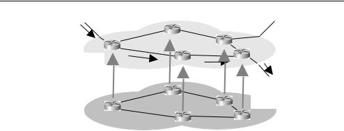
Figure 4.11 illustrates how every router participates both in forwarding packets (on the basis of previously calculated rules) and in performing distributed routing calculations (updating the forwarding rules as necessary).
The detailed art of IP routing is beyond the scope of this book, so we will only briefly summarise a few routing protocols used in the Internet.
4.2.2.1 Shortest-Path Routing
When multiple paths exist between a source and a destination, IP networks use shortestpath routing to pick one particular path. The ‘length’ of a path is typically measured in
52 Networking and Online Games: Understanding and Engineering Multiplayer Internet Games
Forwarding |
|
plane |
|
R3 |
|
R4 |
Routing |
plane |
|
R2 |
|
R1 |
R5 |
|
Figure 4.11 IP routing conceptually consists of separate forwarding and routing functions within each router
terms of hops (the number of routers or links through which the packet passes) but may be defined using any metric desired by the network operator. The path with the lowest ‘sum of metrics over the entire path’ is the shortest path. (for example, in Figure 4.7 the path through R1, R2 and R5 is the shortest path from 136.80.1.2 to 21.80.1.32 when measured by number of router hops.)
Metrics may reflect physical characteristics such as available bandwidth (lower weighting typically given to links with more bandwidth), link delays (higher weighting typically given to links with higher delay) and link costs; or weights may simply represent the administrator’s relative preference for traffic to be on a particular link.
The results of a router’s shortest-path calculations are stored as a set of forwarding rules in a forwarding table, sometimes also referred to as a Forwarding Information Base
(FIB). Forwarding rules specify the appropriate next-hop destinations for packets matching various combinations of network/prefix pairs.
To ensure that routers always utilise the most precisely specified path, they are required to implement a longest prefix match when forwarding packets. In essence, the forwarding table’s entries must be searched for the entry with the longest prefix that matches a packet’s destination. The entry thus discovered is the correct next hop.
The routing protocol may also choose to use (or be required to account for) two extreme network/prefix pairs – default routes and host routes. Default routes are represented by the network/prefix 0.0.0.0/0 – a guaranteed match to any IP address. Because the prefix length is zero, this route is the last entry in a router’s forwarding table.
Default routes are the ultimate in aggregation – if there is only one next-hop link out of the local network, a default route entry can point to that link (instead of having explicit forwarding rules for all the network/prefix pairs that can be reached in the world outside the local network). For example, in Figure 4.7 router R1 would have specific routes pointing into Network 1 for destinations under 128.80/16, and a default route entry pointing out toward the IP Backbone.
Host routes are represented by the network/prefix w.x.y.z/32 – a rule that only matches packets specifically destined for endpoint w.x.y.z. Host routes are discouraged because they are very difficult to aggregate and therefore can consume disproportionate amounts of memory resources in routers throughout the network.
Each destination prefix (whether a network, subnet, or actual host) known to the local network’s routing protocol is said to be the root of its own particular shortest-path tree.
Basic Internet Architecture |
53 |
|
|
The tree has branches passing through every router in the network, although not all links in the network are branches on every shortest-path tree. No matter where a packet appears within the network, the packet will find itself on a branch of a shortest-path tree leading toward its desired destination.
The challenge for a dynamic IP routing protocol is to keep these shortest-path trees current in the presence of router failures, link failures or deliberate modifications to the network’s topology – link failures usually require recalculating the shortest-path trees for many destination prefixes.
4.2.2.2 Autonomous Systems (ASs)
IP networks contain one additional component to their hierarchy – the Autonomous System (AS). An AS is defined loosely as a self-contained, independently administered network or internally connected set of networks. Larger networks, including the Internet itself, can be viewed as an arbitrary topology of interconnected ASs.
The AS exists to provide a bounded scope over which any given routing protocol must track internal topology. Within an AS, routing is managed by Interior Gateway Protocols (IGP, gateway being an old name for routers). Routing of traffic between ASs is managed by an Exterior Gateway Protocol (EGP). The IGP can focus on specific and detailed routes and destinations within the AS, while the EGP deals with summarised information about the AS and networks that can be reached through the AS.
4.2.2.3 Interior Gateway Protocols
Routing protocols that operate within ASs are called IGPs. Distance Vector (DV) and Link State (LS) algorithms have both been used as the basis of IGPs. DV algorithms tend to be simpler to implement, while LS algorithms are more robust when faced with regular topology changes within a network.
DV algorithms require each router to advertise to its neighbours information about the relative distance to each network the router knows (a vector of distances). A router may receive multiple advertisements for the same network X, each from a different neighbour, in which case the router remembers the advertisement with the lowest distance. The neighbour advertising the lowest distance toward X becomes the next hop for packets heading to any destination within network X. The advertising process (typically with intervals in the tens to hundreds of seconds) ensures that information about new networks, or new distances to existing networks, ripples out across the local network whenever changes occur.
LS algorithms distribute maps of the local network’s entire topology (along with the state and metrics of all the links in the topology). The maps are distributed by flooding LS advertisements, whereby each router informs its neighbours about sections of the network topology that the local router knows about. When a state change occurs (for example, a link goes up or down, or a new route is associated with an existing link), the new LS information is flooded across the local network to ensure that all router’s have up-to-date LS maps.
Each router then uses LS maps to locally calculate shortest-path trees to all listed destination networks, and hence determine the appropriate next hops out of the router itself. Because the next-hop calculations are based on complete knowledge of the network’s state, every router can be expected to agree on the shortest-path trees.