Cramer C.J. Essentials of Computational Chemistry Theories and Models

a For atoms, G3 energies are defined to include a spin-orbit correction taken either from experiment or other highlevel calculations. In addition, different coefficients are used in step (8).

b In the G2 method, the 6-311G basis set and its derivatives are not defined for second-row atoms; instead, a basis set optimized by McLean and Chandler (1980) is used.

c Available at http://chemistry.anl.gov/compmat/g3theory.htm. Defined to use canonical 5 d and 7 f functions.

A modification of G2 by Pople and co-workers was deemed sufficiently comprehensive that it is known simply as G3, and its steps are also outlined in Table 7.6. G3 is more accurate than G2, with an error for the 148-molecule heat-of-formation test set of 0.9 kcal mol−1. It is also more efficient, typically being about twice as fast. A particular improvement of G3 over G2 is associated with improved basis sets for the third-row nontransition elements (Curtiss et al. 2001). As with G2, a number of minor to major variations of G3 have been proposed to either improve its efficiency or increase its accuracy over a smaller subset of chemical space, e.g., the G3-RAD method of Henry, Sullivan, and Radom (2003) for particular application to radical thermochemistry, the G3(MP2) model of Curtiss et al. (1999), which reduces computational cost by computing basis-set-extension corrections at the MP2 level instead of the MP4 level, and the G3B3 model of Baboul et al. (1999), which employs B3LYP structures and frequencies.

It should be noted that G2 and G3 potentially fail to be size extensive because of the correction term in step 8. If one is studying a homolytic dissociation into two components, at what point along the reaction coordinate are the formerly paired electrons considered to be unpaired? There will be a discontinuity in the energy at that point. In addition, G3 theory uses a different correction for atoms than for molecules, and this too fails to be size extensive.

Alternative multilevel methods that have some similarities to G2, G3, and their variants, are the CBS methods of Petersson and co-workers (see Bibliography at end of chapter). A key difference between the Gn models and the CBS models is that, rather than assuming basisset incompleteness effects to be completely accounted for by additive corrections, results for different levels of theory are extrapolated to the complete-basis-set limit in defining a composite energy. Four well-defined CBS models exist, CBS-4, CBS-q, CBS-Q, and CBSAPNO, these being in order of increasing accuracy and, naturally, cost. Over the same 148-molecule test set as used above to evaluate G2 and G3, the average absolute errors of CBS-4, CBS-q, and CBS-Q are 2.7, 2.3, and 1.2 kcal mol−1, respectively. CBS-APNO reduces the error in CBS-Q by a factor of 2 (to only 0.5 kcal mol−1 on a somewhat smaller 125-molecule test set), but requires a very expensive QCISD(T)/6-311+G(2df,p) calculation. A particular feature of most of the CBS methods is that they include an (empirical) correction for spin contamination in open-shell species, for which unrestricted treatments potentially sensitive to such contamination are used. In terms of speed, CBS-Q is roughly the speed of G3.

The Weizmann-1 (W1) and Weizmann-2 (W2) models of Martin and de Oliveira (1999) are similar to the CBS models in that extrapolation schemes are used to estimate the infinite basis set limits for SCF and correlation energies. A key difference between the two, however, is that the W1 and W2 models set as a benchmark goal an accuracy of 1 kJ mol−1 (0.24 kcal mol−1 ) on thermochemical quantities. To achieve that kind of accuracy basis sets of size up to cc-pVQZ + 2d1f and cc-pV5Z + 2d1f are used for W1 and W2 theories, respectively, for both SCF and CCSD calculations. Other components of the W1 and W2 calculations include accounting for triple excitations, core electron correlation energy, relativistic effects including spin – orbit coupling, and zero-point vibrational energies. W1 and W2 theories predict heats of formation over a 55-molecule subset of the 148-molecule G2/G3 test set mentioned above (this subset is now usually called the G2-1 test set) with mean unsigned errors of 0.6 and 0.5 kcal mol−1, respectively. By comparison, the G2, G3, and CBS-Q results for this subset are 1.2, 1.1, and 1.0 kcal mol−1, respectively. The relative performances of W1 and W2 theories are still more improved for prediction of electron affinities and ionization potentials (Parthiban and Martin 2001). Further development aimed at achieving ‘spectroscopic accuracy’ (usually defined as energetic accuracy to within 1 cm−1) has resulted in W3 and preliminary W4 theories (Boese et al. 2004), but as these protocols include CCSDTQ calculational steps with basis sets of size cc-pVDZ or larger, they are likely to find application only to very small molecules for the foreseeable future.

A somewhat more obviously empirical variation on the multilevel approach is the multicoefficient method of Truhlar and co-workers. Although many different variations of this approach have now been described, it is simplest to illustrate the concept for the so-called multi-coefficient G3 (MCG3) model (Fast, Sanchez,´ and Truhlar 1999). In essence, the model assumes a G3-like energy expression, but each term has associated with it a coefficient that is not restricted to be unity, as is the case for G3. Specifically

i=1

where (i) represents a component of the G3 energy (actually, there are some rather slight variations involved with basis sets and frozen-core approximations that increase efficiency), ESO and ECC are empirically estimated spin-orbit and core-correlation energies, and the coefficients ci are optimized over the usual G3 thermochemistry test set. One additional important difference in the use of G3 energy components is that the G3 empirical correction, which leads to non-size-extensivity, is not included. Thus, MCG3 is size extensive. The performance of MCG3 is very slightly better than G3 itself, but this accuracy is achieved at roughly half the cost in terms of computational resources for molecules having many heavy atoms. Scaling of the G3 components was also reported by Curtiss et al. (2000) and defines the G3S model. MCG3 and G3S have essentially equivalent accuracy.

The real power in the multi-coefficient models, however, derives from the potential for the coefficients to make up for more severe approximations in the quantities used for (i) in Eq. (7.62). At present, Truhlar and co-workers have codified some 20 different multicoefficient models, some of which they term ‘minimal’, meaning that relatively few terms enter into analogs of Eq. (7.62), and in particular the optimized coefficients absorb the spin-orbit and core-correlation terms, so they are not separately estimated. Different models can thus be chosen for an individual problem based on error tolerance, resource constraints, need to optimize TS geometries at levels beyond MP2, etc. Moreover, for some of the minimal models, analytic derivatives are available on a term-by-term basis, meaning that analytic derivatives for the composite energy can be computed simply as the sum over terms.

A somewhat more chemically based empirical correction scheme is the bond-additivity correction (BAC) methodology. In the BAC-MP4 approach, for instance, the energy of a molecule is computed as

E(BAC-MP4) =E[MP4/6-31G(d,p)//HF/6-31G(d,p)]

where ESC and EMR correct for spin contamination (if any) and multireference character (if any) and the summation runs over all atom pairs and each ‘bond’ correction is a function of bond length (the correction goes to zero at infinite bond length) and a set of parameters, one parameter for each atom and two parameters for each possible pair of atoms. The parameters themselves are determined by fitting to experimental bond dissociation energies, heats of formation (corrected for zero-point vibrational energies and thermal contributions), or other useful thermochemical data. The central assumption of this model, then, is that the error can be decomposed in an additive fashion over the bonds.

In a study of 110 C1 and C2 molecules composed of C, H, O, and F, the average BACMP4 unsigned error in predicted heat of formation was 2.1 kcal mol−1 (Zachariah et al. 1996). As the MP4 calculation uses a relatively modest basis set size, the BAC procedure is quite fast by comparison to some of the multilevel methods described above. On the other hand, as with any method relying on pairwise parameterization, extension to a large number of atoms requires a great deal of parameterization data, and this is a potential limitation of the BAC method when applied to systems containing atoms not already parameterized.

Because they include empirically derived parameters, multilevel models nearly always outperform single-level calculations at an equivalently expensive level of theory. That being said, one should avoid a slavish devotion to any particular multilevel model simply because it has been graced with an acronym defining it. For any given chemical problem, it is quite possible that an individual investigator can construct a specific multilevel model with relatively little effort that will outperform any of the already defined ones. The issue is simply whether sufficient data exist for the particular system of interest in order to make such a focused model possible. When the data do not, then that is the best time to rely on those previously defined models that have been demonstrated to be reasonably robust over relevant swaths of chemical space.

As for the utility of single-level models, it should be recalled that the goal of most multilevel models is absolute energy prediction, while many chemical studies are undertaken in order to better understand relative energy differences. Cancellation of errors makes the latter studies more tractable at less complete levels of theory, and single-level models can still be useful in both qualitative and quantitative senses. In addition, there is no wave function defined for the typical parametric model; there is only an energy functional that potentially depends on several different wave functions. Should one wish to know the expectation value for some property other than the energy, one will either have to devise a separate multilevel expression, or adopt a single-level formalism for which a wave function is indeed defined.

Note that most of the energetic performance data summarized above may also be found in tabular form, compared to density functional models, in Table 8.1

7.8 Case Study: Ethylenedione Radical Anion

Synopsis of Thomas, J. R. et al. (1995) ‘The Ethylenedione Anion: Elucidation of the Intricate Potential Energy Hypersurface’.

The ground state of ethylenedione, the dimer of carbon monoxide, has been reliably predicted to be a triplet that is bound with respect to dissociation by virtue of its high spin state (two singlet carbon monoxide molecules are lower in energy, but the triplet cannot dissociate into two closed-shell singlets). As such, it has proven an interesting target for synthesis, albeit without success. One possible avenue for its synthesis is to detach electrons from negative ion precursors. This prompted Thomas and co-workers to characterize the radical anion of ethylenedione at a variety of correlated levels of electronic structure theory.

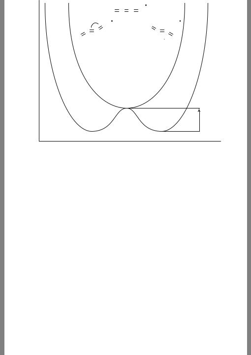
At the UHF level the linear form, which formally has a 2 u electronic state (see Appendix B for details on group theoretical notation), is predicted to be the minimum energy structure. However, at almost all correlated levels the molecule bends to lift the degeneracy of a pair of au and bu orbitals, leading to a so-called Renner – Teller potential energy surface, as illustrated in Figure 7.7. The lower energy state is 2 Au and geometric details are provided in the figure for four different correlated levels, all using a large TZP+ basis set.

The details of the molecular structure are difficult to nail down because of the shallow nature of the PES in the vicinity of the linear form. Thus, even with a fairly complete basis set, there are large disagreements between CISD, CCSD, and CCSD(T), although there is a remarkably good (coincidental) agreement between MP2 and CCSD(T). The situation is

Isotope shifts in the frequencies, however, showed very close agreement between theory and experiment, all data agreeing to within 5% for seven different isotopomers.

The authors did examine whether significant non-dynamical correlation effects complicated the system, but MCSCF calculations with large active spaces failed to identify any configurations other than the dominant one that entered with coefficients in excess of 0.09, suggesting that the use of single-reference methods was well justified. Part of the challenge for this particular system simply derives from its negative charge, which imposes a greater demand on basis-set saturation. In any case, this example illustrates how deceptively difficult it can be to converge solution of the Schrodinger¨ equation even for seemingly simple chemical systems – a mere four heavy atoms.

Bibliography and Suggested Additional Reading

Bartlett, R. J. 2000. ‘Perspective on “On the Correlation Problem in Atomic and Molecular Systems. Calculations of Wavefunction Components in Ursell-type Expansion Using Quantum-field Theoretical Methods”’ Theor. Chem. Acc., 103, 273.

Cioslowski, J., Ed. 2001. Quantum-Mechanical Prediction of Thermochemical Data, Kluwer: Dordrecht. Cramer, C. J. 1998. ‘Bergman, Aza-Bergman, and Protonated Aza-Bergman Cyclizations and Intermediate 2,5-Arynes: Chemistry and Challenges to Computation’ J. Am. Chem. Soc., 120, 6261. Cramer, C. J. and Smith, B. A. 1996. ‘Trimethylenemethane. Comparison of Multiconfiguration Self-

consistent Field and Density Functional Methods for a Non-Kekule´ Hydrocarbon’ J. Phys. Chem. 100, 9664.

Curtiss, L. A., Raghavachari, K., Redfern, P. C., Rassolov, V., and Pople, J. A. 1998. ‘Gaussian-3 (G3) Theory for Molecules Containing First and Second-row Atoms’, J. Chem. Phys. 109, 7764.

Feller, D. and Davidson, E. R. 1990. ‘Basis Sets for Ab Initio Molecular Orbital Calculations and Intermolecular Interactions’ in Reviews in Computational Chemistry , Vol. 1, Lipkowitz, K. B. Boyd, D. B., Eds., VCH: New York, 1.

Hehre, W. J. 1995. Practical Strategies for Electronic Structure Calculations , Wavefunction: Irvine, CA. Hehre, W. J., Radom, L., Schleyer, P. v. R., and Pople, J. A. 1986. Ab Initio Molecular Orbital

Theory , Wiley: New York.

Jensen, F. 1999. Introduction to Computational Chemistry , Wiley: Chichester. Levine, I. N. 2000. Quantum Chemistry , 5th Edn., Prentice Hall: New York.

Lynch, B. J. and Truhlar, D. G. 2003. ‘Robust and Affordable Multicoefficient Methods for Thermochemistry and Thermochemical Kinetics: The MCCM/3 Suite and SAC/3’, J. Phys. Chem. A, 107, 3898.

Martin, J. M. L. 1998. ‘Calibration of Atomization Energies of Small Polyatomics’ in Computational Thermochemistry, ACS Symposium Series, Vol. 677, Irikura, K. K. and Frurip, D. J. Eds., American Chemical Society, Washington, DC, 212.

Petersson, G. A. 1998. ‘Complete Basis-set Thermochemistry and Kinetics’ in Computational Thermochemistry, ACS Symposium Series, Vol. 677, Irikura, K. K. and Frurip, D. J., Eds., American Chemical Society, Washington, DC, 237.

Petersson, G. A., Malick, D. K., Wilson, W. G., Ochterski, J. W., Montgomery, J. A., Jr., and Frisch, M. J. 1998. ‘Calibration and Comparison of the Gaussian-2, Complete Basis Set, and Density Functional Methods for Computational Thermochemistry’ J. Chem. Phys., 109, 10 570.

Slipchenko, L. V. and Krylov, A. I. 2003. ‘Electronic Structure of the Trimethylenemethane Diradical in its Ground and Electronically Excited States: Bonding, Equilibrium Geometries, and Vibrational Frequencies’, J. Chem. Phys., 118, 6874.

Szabo, A. and Ostlund, N. S. 1982. Modern Quantum Chemistry , Macmillan: New York.

Werner, H.-J. 2000. ‘Perspective on “Theory of Self-consistent Electron Pairs. An Iterative Method for Correlated Many-electron Wavefunctions”’ Theor. Chem. Acc., 103, 322.

Zachariah, M. R. and Melius, C. F. 1998. ‘Bond-additivity Correction of Ab Initio Computations for Accurate Prediction of Thermochemistry’ in Computational Thermochemistry , ACS Symposium Series, Vol. 677, Irikura, K. K. and Frurip, D. J., Eds., American Chemical Society, Washington, DC, 162.

References

Abrams, M. L. and Sherrill, C. D. 2003. J. Chem. Phys., 118, 1604. Andersson, K. 1995. Theor. Chim. Acta, 91, 31.

Andersson, K., Malmqvist, P. -A˚ ., and Roos, B. O. 1992. J. Chem. Phys., 96, 1218.

Baboul, A. G., Curtiss, L. A., Redfern, P. C., and Raghavachari, K. 1999. J. Chem. Phys., 110, 7650. Barrows, S. E., Storer, J. W., Cramer, C. J., French, A. D., and Truhlar, D. G. 1998. J. Comput.

Chem., 19, 1111.

Bartlett, R. J. 1981. Ann. Rev. Phys. Chem., 32, 359.

Bartlett, R. J. 1995. In: Modern Electronic Structure Theory , Yarkony, D. R., Ed., World Scientific: New York, Part 2, Chapter 6.

Blomberg, M. R. A. and Siegbahn, P. E. M. 1998. In: Computational Chemistry , ACS Symposium Series, Vol. 677, Irikura, K. K. and Frurip, D. J., Eds., American Chemical Society: Washington, DC, 197.

Boese, A. D., Oren, M., Atasoylu, O., Martin, J. M. L., Kallay,´ M., and Gauss, J. 2004. J. Chem. Phys., 120, 4129.

Brillouin, L. 1934. Actualities Sci. Ind., 71, 159.

Bruna, P. J., Peyerimhoff, S. D., and Buenker, R. J. 1980. Chem. Phys. Lett., 72, 278. Chen, W. and Schlegel, H. B. 1994. J. Chem. Phys., 101, 5957.

Cizek, J. 1966. J. Chem. Phys., 45, 4256.

Crawford, T. D. and Schaefer, H. F., III, 1996. In: Reviews in Computational Chemistry , Vol. 14, Lipkowitz, K. B. and Boyd, D. B., Eds., Wiley-VCH: New York, 33 and references therein.

Curtiss, L. A., Raghavachari, K., and Pople, J. A. 1993. J. Chem. Phys., 98, 1293.

Curtiss, L. A., Raghavachari, K., Redfern, P. C., and Pople, J. A. 2000. J. Chem. Phys., 112, 7374. Curtiss, L. A., Raghavachari, K., Trucks, G. W., and Pople, J. A. 1991. J. Chem. Phys., 94, 7221. Curtiss, L. A., Redfern, P. C., Raghavachari, K., Rassolov, V., and Pople, J. A. 1999. J. Chem. Phys.,

110, 4703.

Curtiss, L. A., Redfern, P. C., Rassolov, V., Kedziora, G., and Pople, J. A. 2001. J. Chem. Phys., 114, 9287.

Davidson, E. R. 1995. Chem. Phys. Lett., 241, 432.

Debbert, S. L. and Cramer, C. J. 2000. Int. J. Mass Spectrom., 201, 1. Dutta, A. and Sherrill, C. D. 2003. J. Chem. Phys., 118, 1610.

Fast, P. L., Sanchez,´ P. L., and Truhlar, D. G. 1999. Chem. Phys. Lett., 306, 407. Feller, D. and Peterson, K. A. 1998. J. Chem. Phys., 108, 154.

Finley, J. P. and Freed, K. F. 1995. J. Chem. Phys., 102, 1306. Gordon, M. S. and Truhlar, D. G. 1986. J. Am. Chem. Soc., 108, 5412. Grimme, S. 2003a. J. Chem. Phys., 118, 9095.

Grimme, S. 2003b. J. Comput. Chem., 24, 1529.

Hald, K., Halkier, A., Jørgensen, P., Coriani, S., Hattig,¨ C., and Helgaker, T. 2003. J. Chem. Phys., 118, 2985.

He, Z. and Cremer, D. 1991. Int. J. Quantum Chem., Quantum Chem. Symp., 25, 43.

248 7 INCLUDING ELECTRON CORRELATION IN MO THEORY

He, Y. and Cremer, D. 2000a. Mol. Phys., 98, 1415.

He, Y. and Cremer, D. 2000b. Theor. Chem. Acc., 105, 110.

He, Y. and Cremer, D. 2000c. J. Phys. Chem. A, 104, 7679.

Head-Gordon, M., Rico, R. J., Oumi, M., and Lee, T. J. 1994. Chem. Phys. Lett., 219, 21.

Helgaker, T., Klopper, W., Halkier, A., Bak, K. L., Jørgensen, P., and Olsen, J. 2001. in Quantum Mechanical Prediction of Thermodynamic Data, Cioslowski, J., Ed., Kluwer: Dordrecht, 1.

Henry, D. J., Sullivan, M. B., and Radom, L. 2003. J. Chem. Phys., 118, 4849. Hylleraas, E. A. 1929. Z. Phys., 54, 347.

Kallay, M. and Gauss, J. 2004. J. Chem. Phys., 120, 6841. Klopper, W. and Kutzelnigg, W. 1987. Chem. Phys. Lett., 134, 17. Krylov, A. I. 2001. Chem. Phys. Lett., 350, 522.

Krylov, A. I. and Sherrill, C. D. 2002. J. Chem. Phys., 116, 3194. Langhoff, S. R. and Davidson, E. R. 1974. Int. J. Quantum Chem., 8, 61. Lee, T. J. and Taylor, P. R. 1989. Int. J. Quantum Chem., S23, 199. Levchenko, S. V. and Krylov, A. I. 2004. J. Chem. Phys., 120, 175.

Li, S. H., Ma, J., and Jiang, Y. S. 2002. J. Comput. Chem., 23, 237. Martin, J. M. L. and de Oliveira, G. 1999. J. Chem. Phys., 111, 1843. McLean, A. D. and Chandler, G. S. 1980. J. Chem. Phys.,72, 5639. Møller, C. and Plesset, M. S. 1934. Phys. Rev., 46, 359.

Page, C. S. and Olivucci, M. 2003. J. Comput. Chem., 24, 298. Parthiban, S. and Martin, J. M. L. 2001. J. Chem. Phys., 114, 6014. Petersson, G. A. and Frisch, M. J. 2000. J. Phys. Chem. A, 104, 2183.

Pitarch-Ruiz, J., Sanchez-Marin, J., and Maynau, D. 2002. J. Comput. Chem., 23, 1157. Pople, J. A., Head-Gordon, M., and Raghavachari, K. 1987. J. Chem. Phys., 87, 5968. Pulay, P. 1983. Chem. Phys. Lett., 100, 151.

Raghavachari, K., Trucks, G. W., Pople, J. A., and Head-Gordon, M. 1989. Chem. Phys. Lett., 157, 479. Saebø, S. and Pulay, P. 1987. J. Chem. Phys., 86, 914.

Scheiner, A. C., Baker, J., and Andzelm, J. W. 1997. J. Comput. Chem., 18, 775. Schutz,¨ M. 2002. Phys. Chem. Chem. Phys., 4, 3941.

Schwartz, C. 1962. Phys. Rev., 126, 1015.

Siegbahn, P. E. M., Blomberg, M. R., and Svensson, M. 1994. Chem. Phys. Lett., 223, 35. Slipchenko, L. V. and Krylov, A. I. 2002. J. Chem. Phys., 117, 4694.

Thomas, J. R., DeLeeuw, B. J., O’Leary, P., Schaefer, H. F., III, Duke, B. J., and O’Leary, B. 1995.

J. Chem. Phys., 102, 652.

Wenthold, P. G., Squires, R. R., and Lineberger, W. C. 1998. J. Am. Chem. Soc., 120, 5279. Woon, D. E. and Dunning, T. H., Jr., 1995 J. Chem. Phys., 103, 4572.

Zachariah, M. R., Westmoreland, P. R., Burgess, D. R., Jr., Tsang, W., and Melius, C. F. 1996. J. Phys. Chem., 100, 8737.

8

Density Functional Theory

8.1Theoretical Motivation

8.1.1Philosophy

What a strange and complicated beast a wave function is. This function, depending on one spin and three spatial coordinates for every electron (assuming fixed nuclear positions), is not, in and of itself, particularly intuitive for systems of more than one electron. Indeed, one might approach the HF approximation as not so much a mathematical tool but more a philosophical one. By allowing the wave function to be expressed as a Slater determinant of one-electron orbitals, one preserves for the chemist some semblance of clarity by permitting each electron still to be thought of as being loosely independent. It was noted in Section 7.6.1 that wave functions can be dramatically improved in quality by removing this rough independence and including in the wave functional form a dependence on interelectronic distances (R12 methods). The key disadvantage? The wave function itself is essentially uninterpretable – it is an inscrutable oracle that returns valuably accurate answers when questioned by quantum mechanical operators, but it offers little by way of sparking intuition.

One may be forgiven for stepping back from the towering edifice of molecular orbital theory and asking, shouldn’t things be simpler? For instance, rather than having to work with a wave function, which has rather odd units of probability density to the one-half power, why can’t we work with some physical observable in determining the energy (and possibly other properties) of a molecule? That such a thing should be possible would probably not have surprised physicists before the discovery of quantum mechanics, insofar as such simple formalisms are widely available in classical systems.

However, we may take advantage of our knowledge of quantum mechanics in asking about what particular physical observable might be useful. Having gone through the exercise of constructing the Hamiltonian operator and showing the utility of its eigenfunctions, it would be sufficient to our task simply to find a physical observable that permitted the a priori construction of the Hamiltonian operator. What then is needed? The Hamiltonian depends only on the positions and atomic numbers of the nuclei and the total number of electrons. The dependence on total number of electrons immediately suggests that a useful physical observable would be the electron density ρ, since, integrated over all space, it gives the total

Essentials of Computational Chemistry, 2nd Edition Christopher J. Cramer

2004 John Wiley & Sons, Ltd ISBNs: 0-470-09181-9 (cased); 0-470-09182-7 (pbk)

Moreover, because the nuclei are effectively point charges, it should be obvious that their positions correspond to local maxima in the electron density (and these maxima are also cusps), so the only issue left to completely specify the Hamiltonian is the assignment of nuclear atomic numbers. It can be shown that this information too is available from the density, since for each nucleus A located at an electron density maximum rA

where Z is the atomic number of A, rA is the radial distance from A, and ρ is the spherically averaged density.

Of course, the arguments above do not provide any simpler formalism for finding the energy. They simply indicate that given a known density, one could form the Hamiltonian operator, solve the Schrodinger¨ equation, and determine the wave functions and energy eigenvalues. Nevertheless, they suggest that some simplifications might be possible.

8.1.2 Early Approximations

Energy is separable into kinetic and potential components. If one decides a priori to try to evaluate the molecular energy using only the electron density as a variable, the simplest approach is to consider the system to be classical, in which case the potential energy components are straightforwardly determined. The attraction between the density and the nuclei is

where r1 and r2 are dummy integration variables running over all space.

The kinetic energy of a continuous charge distribution is less obvious. To proceed, we first introduce the fictitious substance ‘jellium’. Jellium is a system composed of an infinite number of electrons moving in an infinite volume of a space that is characterized by a uniformly distributed positive charge (i.e., the positive charge is not particulate in nature, as it is when represented by nuclei). This electronic distribution, also called the uniform electron gas, has a constant non-zero density. Thomas and Fermi, in 1927, used