

20.7.4.6 Weighted noise power in pWOp
The total weighted intermodulation noise power can be determined from Equation 20.23, where x = all products, (A+B), (A-B), etc.
![]()
20.7.4.7 Determination of unlinearity noise using spectral densities
The problem with Bennett's method is the difficulty of dealing with shaped frequency spectra (pre-emphasis at the output of Line repeaters for instance.)
A method using spectral densities (Bell, 1971) overcomes this difficulty and can be extended to include the shape of the H^ and H across the band.
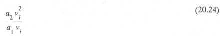
From Equation 20.10 the ratio of the total second order distortion voltage to the fundamental signal at the output of the amplifier or system is given by Equation 20.24, where v is the system input signal (assumed Gaussian).
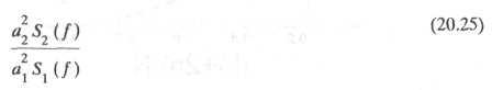
The terms in Equation 20.24 can be expressed as a power in volts squared where S (f) and S (f) are the power spectral densities in volts squared per Hertz. S (f) is the figure for the multichannel input signal voltage, v., and S2(f) for the input signal voltage squared, v?. This is shown in Equation 20.25.
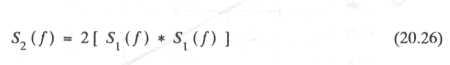
If v is assumed Gaussian then Equation 20.26 may be obtained, ignoring d.c. terms and where represents the convolution integral.
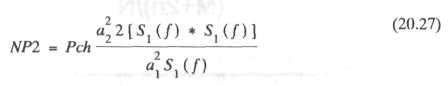
The second order noise power NP2 in watts is therefore given by Equation 20.27, where Pch is the traffic load per channel in watts.
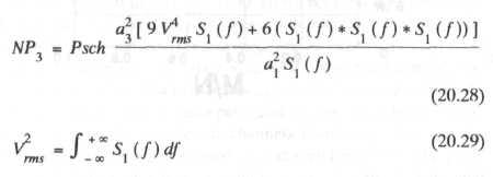
Likewise the third order noise power NP in watts is given by Equation 20.28, where the mean square voltage is given by Equation 20.29 and Pch is the traffic load per channel in watts.
The convolution is best performed numerically on a per system basis.
1 Learn the words & word combinations:
|
Prophometric weighting |
Псофометрическое взвешивание |
|
Weighting factor |
Весовой коэффициент |
|
Gaussian noise |
Нормальный шум |
|
Boltzmann constant |
Постоянная Больцмана |
|
Circuit element |
Элемент цепи |
|
Transmission band |
Полоса пропускания |
|
Activity factor |
Коэффициент активности |
|
Traffic volume |
Интенсивность движения |
|
Trunk network |
Сеть магистральных линий связи |
|
Transfer characteristic |
Переходная характеристика |
|
Multichannel load (multiplexed) |
Информационная нагрузка многоканальной системы |
|
Correction factor |
Поправочный коэффициент Коэффициент исправления |
|
Convolution integral |
Интеграл свертки |
|
Traffic load |
Информационная нагрузка (трафик) |
|
Wire point |
Место присоединения, монтажная точка |
2 Read & translation the text (orally) 20.7:
3 Find Russian equivalents:
|
|
|
|
|
|
|
|
|
|
4 Find English equivalents:
|
|
|
|
|
|
|
|
|
|
|
|
|
|
5 Answer the questions:
What power levels are in common uses?
What is thermal noise?
How can you explain intermodulation or cross modulation noise?
What does the level of the harmonics depend on?
What does the Bennett’s formula explain to calculate?
PART 4 (20.8 – 20.10)
20.8 Measurement of noise contributions
This is also referred to as white noise measurement. Both the thermal noise contributions and the intermodulation noise contributions can be measured directly with one test. This allows rapid field evaluation of installed systems and bench evaluation of individual circuits.
In Figure 20.14 the system is loaded with Gaussian noise from a generating source that has a flat frequency spectrum of noise, bandwidth limited by the filter F .
A single defined channel at frequency f(c) is removed from the spectrum of noise by a filter F before the noise band is transmitted into the system.
A measurement on the same channel at frequency f(c) selected by filter F at the receiver will therefore measure noise that has been generated only within the system itself.
The system is loaded with noise power P that represents the expected multichannel load, as in Equation 20.30, where P The total power of the signal applied to the system, P is the multichannel load for N channels, and T is the transmission level point in dBm.
![]()
For instance, the figures for a 4MHz system at a -3()dBm transmission level point will be P = +14.8dBmO (assuming the normal channel loading of-15dBmO). P will evaluate to-15.2dBm at T = -30dBm.
Two measurements are taken. The first is with the channel stop filter at the transmitter by-passed with the switch S in the closed position. This gives the power due to simulated traffic in a single channel referred to the meter calibration. Measured figure = N .
The second measurement is with the channel stop filter at the transmitter in circuit with the switch S open. This gives the noise power generated from the system referred to the same meter calibration. Measured figure = N .
The Noise Power Ratio (NPR) is given by 101og(Ns/Nn) dB.
The total noise power falling into the channel can be determined from Equation 20.31, where N is the total weighted noise contribution over 4kHz in the specified channel in dBmOp, k = B/4N where B is the bandwidth of the system bandwidth limiting filter in kHz, and N is the number of channels.
![]()
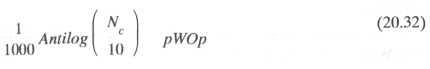
The term l0 log k is to correct for the fact that the actual traffic load has gaps between the channels and is not continuous. The total noise power is also given in pWOp by Equation 20.32.
Several channels are selected for measurement over the band by varying the frequency f(c) of both the channel stop filter in the transmitter and the channel pass filter in the receiver.
Also of interest is to vary the channel loading factor L (nominally -15dBmO) and determine the NPR for various conditions of traffic load. This is a measure of the system's robustness to peak loads and transmission level changes outside the normal design guides. The normal expected NPR curve is shown in Figure 20.15.
As the transmission load is lowered then the basic or Gaussian noise predominates. The NPR increases linearly with decreasing traffic power. As the transmission load is increased then intermodu-lation noise predominates and the NPR rapidly rises as more higher order intermodulation products contribute.
The optimum working point of the system is easily determined from Figure 20.15