

Week 6: Vector Torque and Angular Momentum |
|
|
289 |
|
or |
r1 |
|
|
|
v2 = |
v1 |
(598) |
||
|
||||
|
r2 |
|
||
f)Compute the work done by the force from part c) above and identify the answer as the workkinetic energy theorem. Use this to to find the velocity v2. You should get the same answer! Well, what can we do but follow instructions. L and m are constants and we can take them
~
right out of the integral as soon as they appear. Note that dr points out and F points in along r so that:
W = |
−Zr1 |
2 |
F dr |
||||||||||
|
|
|
|
|
|
r |
|
|
|
|
|
|
|
= |
−Zr1 |
|
|
|
mr3 dr |
||||||||
|
|
|
|
|
|
r2 |
|
L2 |
|||||
= |
− m |
|
Zr1 |
|
r−3dr |
||||||||
|
|
|
L2 |
|
|
|
|
r2 |
|||||
= |
|
m |
|
2 |
|
¯r1 |
|||||||
|
L2 r−2 |
¯ |
r2 |
||||||||||
|
|
|
|
|
|
|
|
|
¯ |
|
L2 |
||
|
|
L2 |
|
|
|
|
|
||||||
= |
|
|
|
|
|
|
|
|
|
¯ |
|
|
|
|
|
|
|
|
|
|
|
|
|
|
|
||
|
2mr22 − 2mr12 |
||||||||||||
= |
|
K |
|
|
|
|
|
(599) |
|||||
Not really so di cult after all.
Note that the last two results are pretty amazing – they show that our torque and angular momentum theory so far is remarkably consistent since two very di erent approaches give the same answer. Solving this problem now will make it easy later to understand the angular momentum barrier, the angular kinetic energy term that appears in the radial part of conservation of mechanical energy in problems involving a central force (such as gravitation and Coulomb’s Law). This in turn will make it easy for us to understand certain properties of orbits from their potential energy curves.
The final application of the Law of Conservation of Angular Momentum, collisions in this text is too important to be just a subsection – it gets its very own topical section, following immediately.
6.5: Collisions
We don’t need to dwell too much on the general theory of collisions at this point – all of the definitions of terms and the general methodology we learned in week 4 still hold when we allow for rotations. The primary di erence is that we can now apply the Law of Conservation of Angular Momentum as well as the Law of Conservation of Linear Momentum to the actual collision impulse.
In particular, in collisions where no external force acts (in the impulse approximation), no external torque can act as well. In these collisions both linear momentum and angular momentum are conserved by the collision. Furthermore, the angular momentum can be computed relative to any pivot, so one can choose a convenient pivot to simply the algebra involved in solving any given problem.
This is illustrated in figure 84 above, where a small disk collides with a bar, both sitting (we imagine) on a frictionless table so that there is no net external force or torque acting. Both momentum and angular momentum are conserved in this collision. The most convenient pivot for problems of this sort is usually the center of mass of the bar, or possibly the center of mass of the system at the instant of collision (which continues moving a the constant speed of the center of mass before the collision, of course).
290 Week 6: Vector Torque and Angular Momentum
M M
m |
v |
m |
|
Figure 84: In the collision above, no physical pivot exist and hence no external force or torque is exerted during the collision. In collisions of this sort both momentum and angular momentum about any pivot chosen are conserved.
All of the terminology developed to describe the energetics of di erent collisions still holds when we consider conservation of angular momentum in addition to conservation of linear momentum. Thus we can speak of elastic collisions where kinetic energy is conserved during the collision, and partially or fully inelastic collisions where it is not, with “fully inelastic” as usual being a collision where the systems collide and stick together (so that they have the same velocity of and angular velocity around the center of mass after the collision).
|
pivot |
M |
M |
|
m v |
m |
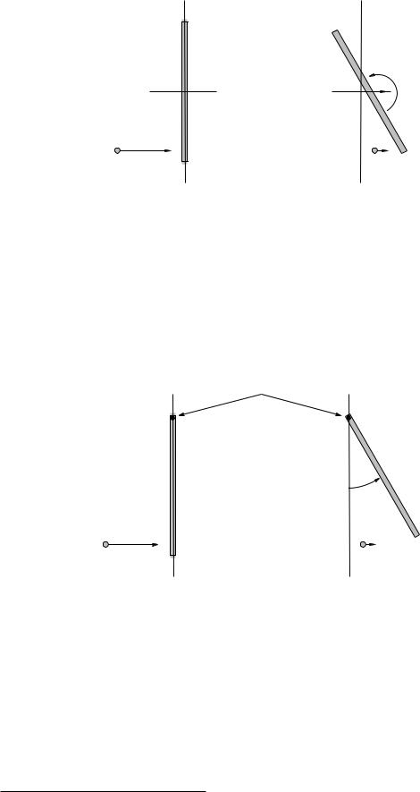
Figure 85: In the collision above, a physical pivot exists – the bar has a hinge at one end that prevents its linear motion while permitting the bar to swing freely. In collisions of this sort linear momentum is not conserved, but since the pivot force exerts no torque about the pivot, angular momentum about the pivot is conserved.
We do, however, have a new class of collision that can occur, illustrated in figure 85, one where the angular momentum is conserved but linear momentum is not. This can and in general will occur when a system experiences a collision where a certain point in the system is physically pivoted by means of a nail, an axle, a hinge so that during the collision an unknown force119 is exerted there as an extra external “impulse” acting on the system. This impulse acting at the pivot exerts no external torque around the pivot so angular momentum relative to the pivot is conserved but linear momentum is, alas, not conserved in these collisions.
119Often we can actually evaluate at least the impulse imparted by such a pivot during the collision – it is “unknown” in that it is usually not given as part of the initial data.
Week 6: Vector Torque and Angular Momentum |
291 |
It is extremely important for you to be able to analyze any given problem to identify the conserved quantities. To help you out, I’ve made up a a wee “collision type” table, where you can look for the term “elastic” in the problem – if it isn’t explicitly there, by default it is at least partially inelastic unless/until proven otherwise during the solution – and also look to see if there is a pivot force that again by default prevents momentum from being conserved unless/until proven otherwise during the solution.
|
Pivot Force |
No Pivot Force |
|
|
|
|
|
Elastic |
~ |
~ |
~ |
K, L conserved |
K, L and P conserved. |
||
Inelastic |
~ |
~ |
~ |
L conserved |
L and P conserved. |
||
Table 4: Table to help you categorize a collision problem so that you can use the correct conservation laws to try to solve it. Note that you can get over half the credit for any given problem simply by correctly identifying the conserved quantities even if you then completely screw up the algebra.
The best way to come to understand this table (and how to proceed to add angular momentum conservation to your repertoire of tricks for analyzing collisions) is by considering the following examples. I’m only doing part of the work of solving them here, so you can experience the joy of solving them the rest of the way – and learning how it all goes – for homework.
We’ll start with the easiest collisions of this sort to solve – fully inelastic collisions.
Example 6.5.1: Fully Inelastic Collision of Ball of Putty with a Free Rod
M |
|
M |
xcm |
|
|
|
L |
ω f |
|
|
|
|
|
vf |
|
|
m |
m v0
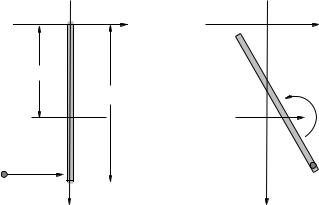
Figure 86: A blob of putty of mass m, travelling at initial velocity v0 to the right, strikes an unpivoted rod of mass M and length L at the end and sticks to it. No friction or external forces act on the system.
In figure 86 a blob of putty of mass m strikes a stationary rod of mass M at one end and sticks. The putty and rod recoil together, rotating around their mutual center of mass. Everything is in a vacuum in a space station or on a frictionless table or something like that – in any event there are no other forces acting during the collision or we ignore them in the impulse approximation.
First we have to figure out the physics. We mentally examine our table of possible collision types. There is no pivot, so there are no relevant external forces. No external force, no external torque, so both momentum and angular momentum are conserved by this collision. However, it is a fully inelastic collision so that kinetic energy is (maximally) not conserved.
Typical questions are:
• Where is the center of mass at the time of the collision (what is xcm)?
292 |
Week 6: Vector Torque and Angular Momentum |
•What is vf , the speed of the center of mass after the collision? Note that if we know the answer to these two questions, we actually know xcm(t) for all future times!
•What is ωf , the final angular velocity of rotation around the center of mass? If we know this, we also know θ(t) and hence can precisely locate every bit of mass in the system for all times after the collision.
•How much kinetic energy is lost in the collision, and where does it go?
We’ll answer these very systematically, in this order. Note well that for each answer, the physics knowledge required is pretty simple and well within your reach – it’s just that there are a lot of parts to patiently wade through.
To find xcm: |
|
L |
|
|
||
(M + m)xcm = M |
+ mL |
(600) |
||||
|
|
|||||
2 |
||||||
or |
M/2 + m |
|
|
|||
xcm = |
L |
(601) |
||||
|
||||||
M + m |
||||||
where I’m taking it as “obvious” that the center of mass of the rod itself is at L/2.
To find vf , we note that momentum is conserved (and also recall that the answer is going to be
vcm:
pi = mv0 = (M + m)vf = pf |
(602) |
||
or |
m |
|
|
vf = vcm = |
|
||
|
v0 |
(603) |
|
M + m |
|||
To find ωf , we note that angular momentum is going to be conserved. This is where we have to start to actually think a bit – I’m hoping that the previous two solutions are really easy for you at this point as we’ve seen each one (and worked through them in detail) at least a half dozen to a dozen times on homework and examples in class and in this book.
First of all, the good news. The rotation of ball and rod before and after the collision all happens in the plane of rotation, so we don’t have to mess with anything but scalar moments of inertia and L = Iω. Then, the bad news: We have to choose a pivot since none was provided for us. The answer will be the same no matter which pivot you choose, but the algebra required to find the answer may be quite di erent (and more di cult for some choices).
Let’s think for a bit. We know the standard scalar moment of inertia of the rod (which applies in this case) around two points – the end or the middle/center of mass. However, the final rotation is around not the center of mass of the rod but the center of mass of the system, as the center of mass of the system itself moves in a completely straight line throughout.
Of course, the angular velocity is the same regardless of our choice of pivot. We could choose the end of the rod, the center of the rod, or the center of mass of the system and in all cases the final angular momentum will be the same, but unless we choose the center of mass of the system to be our pivot we will have to deal with the fact that our final angular momentum will have both a translational and a rotational piece.
This suggests that our “best choice” is to choose xcm as our pivot, eliminating the translational angular momentum altogether, and that is how we will proceed. However, I’m also going to solve this problem using the upper end of the rod at the instant of the collision as a pivot, because I’m quite certain that no student reading this yet understands what I mean about the translational component of the angular momentum!
Using xcm:

Week 6: Vector Torque and Angular Momentum |
293 |
We must compute the initial angular momentum of the system before the collision. This is just the angular momentum of the incoming blob of putty at the instant of collision as the rod is at rest.
Li = |~r × p~| = mv0r = mv0(L − xcm) |
(604) |
Note that the “moment arm” of the angular momentum of the mass m in this frame is just the perpendicular minimum distance from the pivot to the line of motion of m, L − xcm.
This must equal the final angular momentum of the system. This is easy enough to write down:
Li = mv0(L − xcm) = If ωf = Lf |
(605) |
where If is the moment of inertia of the entire rotating system about the xcm pivot!
Note well: The advantage of using this frame with the pivot at xcm at the instant of collision (or any other frame with the pivot on the straight line of motion of xcm) is that in this frame the angular momentum of the system treated as a mass at the center of mass is zero. We
~
only have a rotational part of L in any of these coordinate frames, not a rotational and translational part. This makes the algebra (in my opinion) very slightly simpler in this frame than in, say, the frame with a pivot at the end of the rod/origin illustrated next, although the algebra in the the frame with pivot at the origin almost instantly “corrects itself” and gives us the center of mass pivot result.
This now reveals the only point where we have to do real work in this frame (or any other) – finding If around the center of mass! Lots of opportunities to make mistakes, a need to use Our Friend, the Parallel Axis Theorem, alarums and excursions galore. However, if you have clearly stated Li = Lf , and correctly represented them as in the equation above, you have little to fear – you might lose a point if you screw up the evaluation of If , you might even lose two or three, but that’s out of 10 to 25 points total for the problem – you’re already way up there as far as your demonstrated knowledge of physics is concerned!
So let’s give it a try. The total moment of intertia is the moment of inertia of the rod around the new (parallel) axis through xcm plus the moment of inertia of the blob of putty as a “point mass” stuck on at the end. Sounds like a job for the Parallel Axis Theorem!
|
1 |
|
If = |
12 M L2 + M (xcm − L/2)2 + m(L − xcm)2 |
(606) |
Now be honest; this isn’t really that hard to write down, is it?
Of course the “mess” occurs when we substitute this back into the conservation of momentum equation and solve for ωf :
ωf = |
Li |
= |
|
|
mv0(L − xcm) |
(607) |
|
|
1 |
M L2 + M (xcm − L/2)2 + m(L − xcm)2 |
|||
|
If |
|
|
|||
|
|
12 |
|
|||
One could possible square out everything in the denominator and “simplify” this, but why would one want to? If we know the actual numerical values of m, M , L, and v0, we can compute (in order) xcm, If and ωf as easily from this expression as from any other, and this expression actually means something and can be checked at a glance by your instructors. Your instructors would have to work just as hard as you would to reduce it to minimal terms, and are just as averse to doing pointless work.
That’s not to say that one should never multiply things out and simplify, only that it seems unreasonable to count doing so as being part of the physics of the “answer”, and all we really care about is the physics! As a rule in this course, if you are a math, physics, or engineering major I expect you to go the extra mile and finish o the algebra, but if you are a life science major who came into the course terrified of anything involving algebra, well, I’m proud of you already because by