copy it or refer to it. If you choose to copy our example, make sure you learn what each of its commands is doing by consulting the Octave documentation.

%Find Indices of Positive and Negative Examples pos = find(y==1); neg = find(y == 0);

%Plot Examples

plot(X(pos, 1), X(pos, 2), 'k+','LineWidth', 2, ...

'MarkerSize', 7);

plot(X(neg, 1), X(neg, 2), 'ko', 'MarkerFaceColor', 'y', ...

'MarkerSize', 7);

1.2Implementation

1.2.1Warmup exercise: sigmoid function

Before you start with the actual cost function, recall that the logistic regression hypothesis is defined as:

hθ(x) = g(θT x),

where function g is the sigmoid function. The sigmoid function is defined as:

1 g(z) = 1 + e−z .

Your first step is to implement this function in sigmoid.m so it can be called by the rest of your program. When you are finished, try testing a few values by calling sigmoid(x) at the octave command line. For large positive values of x, the sigmoid should be close to 1, while for large negative values, the sigmoid should be close to 0. Evaluating sigmoid(0) should give you exactly 0.5. Your code should also work with vectors and matrices. For a matrix, your function should perform the sigmoid function on every element.

You can submit your solution for grading by typing submit at the Octave command line. The submission script will prompt you for your username and password and ask you which files you want to submit. You can obtain a submission password from the website.

You should now submit the warm up exercise.

4

1.2.2Cost function and gradient

Now you will implement the cost function and gradient for logistic regression. Complete the code in costFunction.m to return the cost and gradient.

Recall that the cost function in logistic regression is

m

J(θ) = m1 X −y(i) log(hθ(x(i))) − (1 − y(i)) log(1 − hθ(x(i))) ,

i=1

and the gradient of the cost is a vector of the same length as θ where the jth element (for j = 0, 1, . . . , n) is defined as follows:

Note that while this gradient looks identical to the linear regression gradient, the formula is actually di erent because linear and logistic regression have di erent definitions of hθ(x).

Once you are done, ex2.m will call your costFunction using the initial parameters of θ. You should see that the cost is about 0.693.

You should now submit the cost function and gradient for logistic regression. Make two submissions: one for the cost function and one for the gradient.

1.2.3Learning parameters using fminunc

In the previous assignment, you found the optimal parameters of a linear regression model by implementing gradent descent. You wrote a cost function and calculated its gradient, then took a gradient descent step accordingly. This time, instead of taking gradient descent steps, you will use an Octave built-in function called fminunc.

Octave’s fminunc is an optimization solver that finds the minimum of an unconstrained2 function. For logistic regression, you want to optimize the cost function J(θ) with parameters θ.

2Constraints in optimization often refer to constraints on the parameters, for example, constraints that bound the possible values θ can take (e.g., θ ≤ 1). Logistic regression does not have such constraints since θ is allowed to take any real value.

5

Concretely, you are going to use fminunc to find the best parameters θ for the logistic regression cost function, given a fixed dataset (of X and y values). You will pass to fminunc the following inputs:

The initial values of the parameters we are trying to optimize.

A function that, when given the training set and a particular θ, computes the logistic regression cost and gradient with respect to θ for the dataset (X, y)

In ex2.m, we already have code written to call fminunc with the correct arguments.

%Set options for fminunc

options = optimset('GradObj', 'on', 'MaxIter', 400);

%Run fminunc to obtain the optimal theta

%This function will return theta and the cost [theta, cost] = ...

fminunc(@(t)(costFunction(t, X, y)), initial theta, options);

In this code snippet, we first defined the options to be used with fminunc. Specifically, we set the GradObj option to on, which tells fminunc that our function returns both the cost and the gradient. This allows fminunc to use the gradient when minimizing the function. Furthermore, we set the MaxIter option to 400, so that fminunc will run for at most 400 steps before it terminates.

To specify the actual function we are minimizing, we use a “short-hand” for specifying functions with the @(t) ( costFunction(t, X, y) ) . This creates a function, with argument t, which calls your costFunction. This allows us to wrap the costFunction for use with fminunc.

If you have completed the costFunction correctly, fminunc will converge on the right optimization parameters and return the final values of the cost and θ. Notice that by using fminunc, you did not have to write any loops yourself, or set a learning rate like you did for gradient descent. This is all done by fminunc: you only needed to provide a function calculating the cost and the gradient.

Once fminunc completes, ex2.m will call your costFunction function using the optimal parameters of θ. You should see that the cost is about 0.203.

This final θ value will then be used to plot the decision boundary on the training data, resulting in a figure similar to Figure 2. We also encourage

6

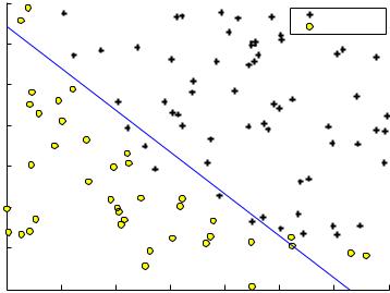
you to look at the code in plotDecisionBoundary.m to see how to plot such a boundary using the θ values.

Exam 1 score

Figure 2: Training data with decision boundary

1.2.4Evaluating logistic regression

After learning the parameters, you can use the model to predict whether a particular student will be admitted. For a student with an Exam 1 score of 45 and an Exam 2 score of 85, you should expect to see an admission probability of 0.776.

Another way to evaluate the quality of the parameters we have found is to see how well the learned model predicts on our training set. In this part, your task is to complete the code in predict.m. The predict function will produce “1” or “0” predictions given a dataset and a learned parameter vector θ.

After you have completed the code in predict.m, the ex2.m script will proceed to report the training accuracy of your classifier by computing the percentage of examples it got correct.

You should now submit the prediction function for logistic regression.

7