Психология

task. In these cases people who score higher on one of the variables tend to score lower on the other variable.

Relationships between variables that cannot be described with a straight line are known

as nonlinear relationships. Part (c) of Figure 2.10 "Examples of Scatter Plots" shows a common pattern in which the distribution of the points is essentially random. In this case there is no relationship at all between the two variables, and they are said to be independent. Parts (d) and

(e) of Figure 2.10 "Examples of Scatter Plots" show patterns of association in which, although there is an association, the points are not well described by a single straight line. For instance, part (d) shows the type of relationship that frequently occurs between anxiety and performance. Increases in anxiety from low to moderate levels are associated with performance increases, whereas increases in anxiety from moderate to high levels are associated with decreases in performance. Relationships that change in direction and thus are not described by a single straight line are called curvilinear relationships.

Figure 2.10 Examples of Scatter Plots

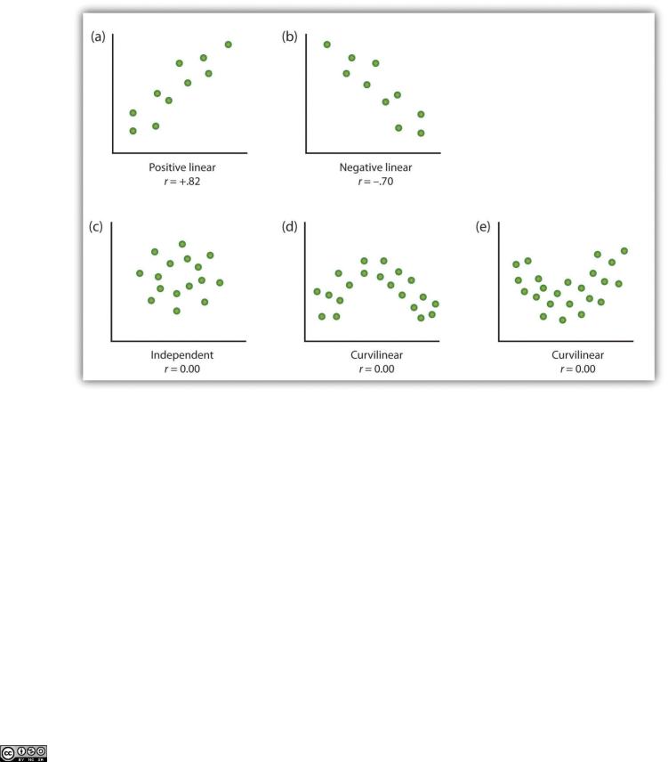
Some examples of relationships between two variables as shown in scatter plots. Note that the Pearson correlation coefficient (r) between variables that have curvilinear relationships will likely be close to zero.

Source: Adapted from Stangor, C. (2011). Research methods for the behavioral sciences (4th ed.). Mountain View, CA: Cengage.

The most common statistical measure of the strength of linear relationships among variables is the Pearson correlation coefficient, which is symbolized by the letter r. The value of the correlation coefficient ranges from r= –1.00 to r = +1.00. The direction of the linear relationship is indicated by the sign of the correlation coefficient. Positive values of r (such as r = .54 or r =

.67) indicate that the relationship is positive linear (i.e., the pattern of the dots on the scatter plot runs from the lower left to the upper right), whereas negative values of r (such as r = –.30 or r = –.72) indicate negative linear relationships (i.e., the dots run from the upper left to the lower

right). The strength of the linear relationship is indexed by the distance of the correlation coefficient from zero (its absolute value). For instance, r = –.54 is a stronger relationship than r=

.30, and r = .72 is a stronger relationship than r = –.57. Because the Pearson correlation coefficient only measures linear relationships, variables that have curvilinear relationships are not well described by r, and the observed correlation will be close to zero.

It is also possible to study relationships among more than two measures at the same time. A research design in which more than one predictor variable is used to predict a single outcome variable is analyzed through multiple regression(Aiken & West,

1991). [6] Multiple regression is a statistical technique, based on correlation coefficients among variables, that allows predicting a single outcome variable from more than one predictor variable. For instance, Figure 2.11 "Prediction of Job Performance From Three Predictor Variables" shows a multiple regression analysis in which three predictor variables are used to predict a single outcome. The use of multiple regression analysis shows an important advantage of correlational research designs—they can be used to make predictions about a person’s likely score on an outcome variable (e.g., job performance) based on knowledge of other variables.

Figure 2.11 Prediction of Job Performance From Three Predictor Variables

Multiple regression allows scientists to predict the scores on a single outcome variable using more than one predictor variable.

An important limitation of correlational research designs is that they cannot be used to draw conclusions about the causal relationships among the measured variables. Consider, for instance, a researcher who has hypothesized that viewing violent behavior will cause increased aggressive play in children. He has collected, from a sample of fourth-grade children, a measure of how many violent television shows each child views during the week, as well as a measure of how aggressively each child plays on the school playground. From his collected data, the researcher discovers a positive correlation between the two measured variables.

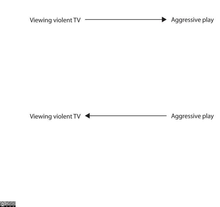
Although this positive correlation appears to support the researcher’s hypothesis, it cannot be taken to indicate that viewing violent television causes aggressive behavior. Although the researcher is tempted to assume that viewing violent television causes aggressive play,

Figure 2.2.2

there are other possibilities. One alternate possibility is that the causal direction is exactly opposite from what has been hypothesized. Perhaps children who have behaved aggressively at school develop residual excitement that leads them to want to watch violent television shows at home:

Figure 2.2.2

Although this possibility may seem less likely, there is no way to rule out the possibility of such reverse causation on the basis of this observed correlation. It is also possible that both causal directions are operating and that the two variables cause each other:

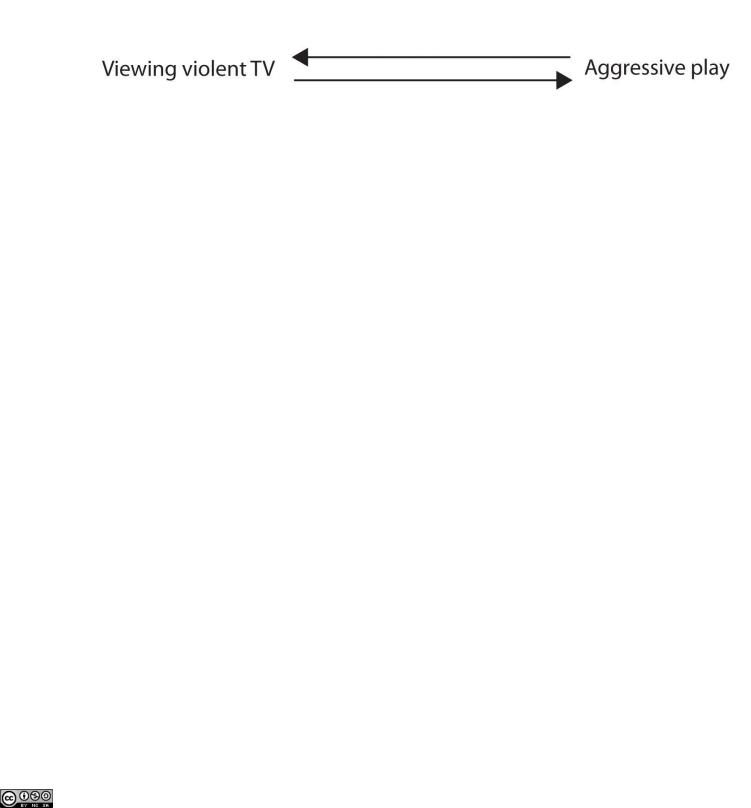
Figure 2.2.2

Still another possible explanation for the observed correlation is that it has been produced by the presence of a common-causal variable (also known as a third variable). A common-

causal variable is a variable that is not part of the research hypothesis but that causes both the predictor and the outcome variable and thus produces the observed correlation between them. In our example a potential common-causal variable is the discipline style of the children’s parents. Parents who use a harsh and punitive discipline style may produce children who both like to watch violent television and who behave aggressively in comparison to children whose parents use less harsh discipline:

Figure 2.2.2

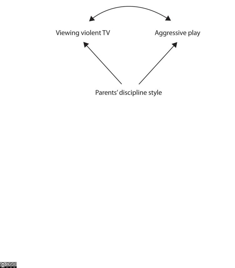
In this case, television viewing and aggressive play would be positively correlated (as indicated by the curved arrow between them), even though neither one caused the other but they were both caused by the discipline style of the parents (the straight arrows). When the predictor and outcome variables are both caused by a common-causal variable, the observed relationship between them is said to be spurious. A spurious relationship is a relationship between two variables in which a common-causal variable produces and “explains away‖ the relationship. If effects of the common-causal variable were taken away, or controlled for, the relationship between the predictor and outcome variables would disappear. In the example the relationship between aggression and television viewing might be spurious because by controlling for the effect of the parents’ disciplining style, the relationship between television viewing and aggressive behavior might go away.

Common-causal variables in correlational research designs can be thought of as “mystery‖ variables because, as they have not been measured, their presence and identity are usually unknown to the researcher. Since it is not possible to measure every variable that could cause both the predictor and outcome variables, the existence of an unknown common-causal variable is always a possibility. For this reason, we are left with the basic limitation of correlational

research: Correlation does not demonstrate causation. It is important that when you read about correlational research projects, you keep in mind the possibility of spurious relationships, and be sure to interpret the findings appropriately. Although correlational research is sometimes reported as demonstrating causality without any mention being made of the possibility of reverse causation or common-causal variables, informed consumers of research, like you, are aware of these interpretational problems.

In sum, correlational research designs have both strengths and limitations. One strength is that they can be used when experimental research is not possible because the predictor variables cannot be manipulated. Correlational designs also have the advantage of allowing the researcher to study behavior as it occurs in everyday life. And we can also use correlational designs to make predictions—for instance, to predict from the scores on their battery of tests the success of job trainees during a training session. But we cannot use such correlational information to determine whether the training caused better job performance. For that, researchers rely on experiments.

Experimental Research: Understanding the Causes of Behavior

The goal of experimental research design is to provide more definitive conclusions about the causal relationships among the variables in the research hypothesis than is available from correlational designs. In an experimental research design, the variables of interest are called the independent variable(or variables) and the dependent variable. The independent variable in an experiment is the causing variable that is created (manipulated) by the experimenter.

The dependent variable in an experiment is a measured variable that is expected to be influenced by the experimental manipulation. The research hypothesis suggests that the manipulated independent variable or variables will cause changes in the measured dependent variables. We can diagram the research hypothesis by using an arrow that points in one direction. This demonstrates the expected direction of causality:

Figure 2.2.3

Research Focus: Video Games and Aggression

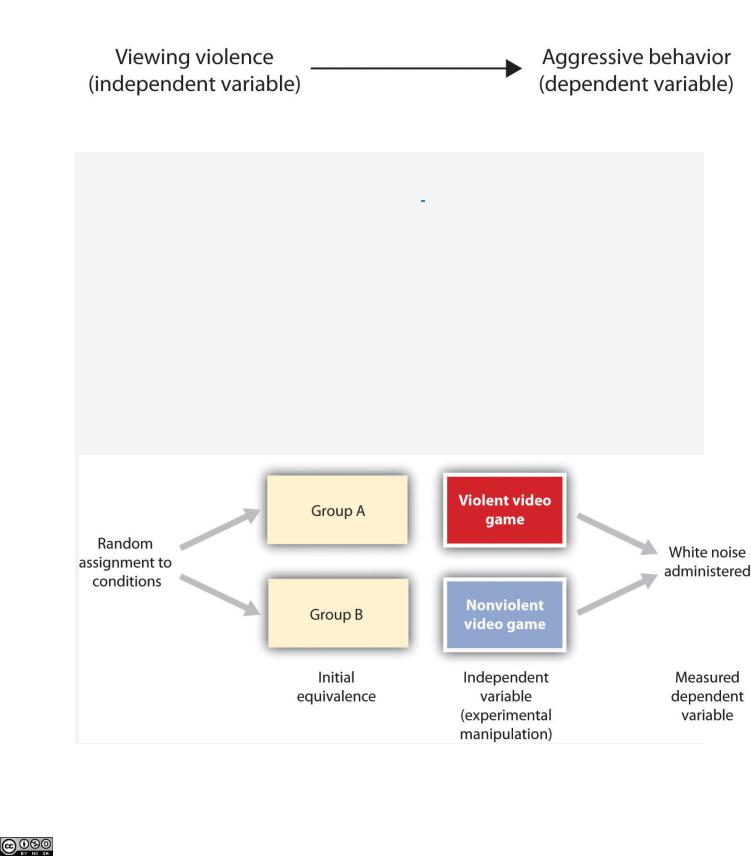
Consider an experiment conducted by Anderson and Dill (2000). [7] The study was designed to test the hypothesis that viewing violent video games would increase aggressive behavior. In this research, male and female undergraduates from Iowa State University were given a chance to play with either a violent video game (Wolfenstein 3D) or a nonviolent video game (Myst). During the experimental session, the participants played their assigned video games for 15 minutes. Then, after the play, each participant played a competitive game with an opponent in which the participant could deliver blasts of white noise through the earphones of the opponent. The operational definition of the dependent variable (aggressive behavior) was the level and duration of noise delivered to the opponent. The design of the experiment is shown in Figure 2.17 "An Experimental Research Design".

Figure 2.17An Experimental Research Design

Two advantages of the experimental research design are (1) the assurance that the independent variable (also known as the experimental manipulation) occurs prior to the measured dependent variable, and (2) the creation of initial equivalence between the conditions of the experiment (in this case by using random assignment to conditions).

Experimental designs have two very nice features. For one, they guarantee that the independent variable occurs prior to the measurement of the dependent variable. This eliminates the possibility of reverse causation. Second, the influence of common-causal variables is controlled, and thus eliminated, by creating initial equivalence among the participants in each of the experimental conditions before the manipulation occurs.

The most common method of creating equivalence among the experimental conditions is

through random assignment to conditions, a procedure in which the condition that each participant is assigned to is determined through a random process, such as drawing numbers out of an envelope or using a random number table. Anderson and Dill first randomly assigned about 100 participants to each of their two groups (Group A and Group B). Because they used random assignment to conditions, they could be confident that, before the experimental manipulation occurred, the students in Group A were, on average, equivalent to the students in Group B on every possible variable, including variables that are likely to be related to aggression, such as parental discipline style, peer relationships, hormone levels, diet—and in fact everything else.

Then, after they had created initial equivalence, Anderson and Dill created the experimental manipulation—they had the participants in Group A play the violent game and the participants in Group B play the nonviolent game. Then they compared the dependent variable (the white noise blasts) between the two groups, finding that the students who had viewed the violent video game gave significantly longer noise blasts than did the students who had played the nonviolent game.

Anderson and Dill had from the outset created initial equivalence between the groups. This initial equivalence allowed them to observe differences in the white noise levels between the two groups after the experimental manipulation, leading to the conclusion that it was the independent variable (and not some other variable) that caused these differences. The idea is that the only thing that was different between the students in the two groups was the video game they had played.