

gpss_manual
.pdf4.17.4 Higher Order Equations
You must reduce the order of higher order ordinary differential equations. If you have higher order differential equations, before you enter them into GPSS World, you should rewrite them as a system of first order equations. This is relatively easy, and requires that you introduce a new variable for each of the intermediate derivatives.
For example, if you have
25 y’’’ - 6 y’ + y = 0.
Let
u = y ‘ v = u ‘ = y’’
For even higher orders, we would continue to introduce variables.
Then, substituting into the original equation and using only one first order derivative, we have
25 v’ - 6 u + y = 0.
Now we have the following system of equations: y’ = u
u’ = v
v’ = 6/25 u - 1/25 y
In GPSS World, you could use the following Statements
Y_ INTEGRATE U_
U_ INTEGRATE V_
V_ INTEGRATE ( (6/25) # U_ - (1/25) # Y_)
To these, you must add EQU Statements that initialize U_, V_, and Y_
4.17.5. Continuous Only
If you want to do a purely continuous simulation, you still need to create a termination condition by entry into a TERMINATE Block. Therefore, include a GPSS segment such as
GENERATE End_Time TERMINATE 1
In the model, which is begun by a
START 1
4.17.6. Phases
Simulations run in alternate continuous and discrete phases. At any instant where events are scheduled, the simulation runs in a discrete phase. The clock does not advance within an instant in a discrete phase. Between instants, the simulation runs in a continuous phase, during which the integrations proceed in small time increments called ministeps. Plotted integration variables report intermediate values at the end of ministeps.
When a threshold crossing generates a Transaction, the simulation goes into a discrete phase. In this manner, the continuous and the discrete phases can be closely interrelated. Conversely, User Variables can be assigned new values in a discrete phase even if they are being integrated. You can do so using an EQU Command, or a PLUS Assignment Statement. If you want such assignments to occur within the running of the simulation, you must define a PLUS Procedure that makes the assignment. For example, if you defined a PLUS Procedure as
PROCEDURE SetPop(Pop_Level)Foxes
= Pop_Level ;
you could reinitialize the FOXES User Variable by entering a PLUS Block, such as
PLUS (SetPop(200))
or by using a parenthesized Expression that invokes SetPop( ) in some other kind of Block.
4.17.7. Integration Error
A Model Setting called the Integration Tolerance is used to limit the local truncation error of integrations. This setting applies to all integrations performed during the simulation. If you make the tolerance smaller, the integrations will take longer, but will be more accurate. This is set in the Simulate Page of the Model Settings Notebook.
CHOOSE View / Settings / Model
Then select the Simulate page. Then fill in the desired value in the entry box marked "Integration Tolerance". The installation default is 10-6.
4.17.8. Related Command
∙ INTEGRATE Commands set up automatic integrations.
4.17.7. Related Block
∙ INTEGRATION Blocks turn the integration of variables ON or OFF.
Chapter 5 - GPSS World Windows
This chapter is a display of all the major windows in GPSS World. The general operation of GPSS World is described in Chapter 2 of this manual.
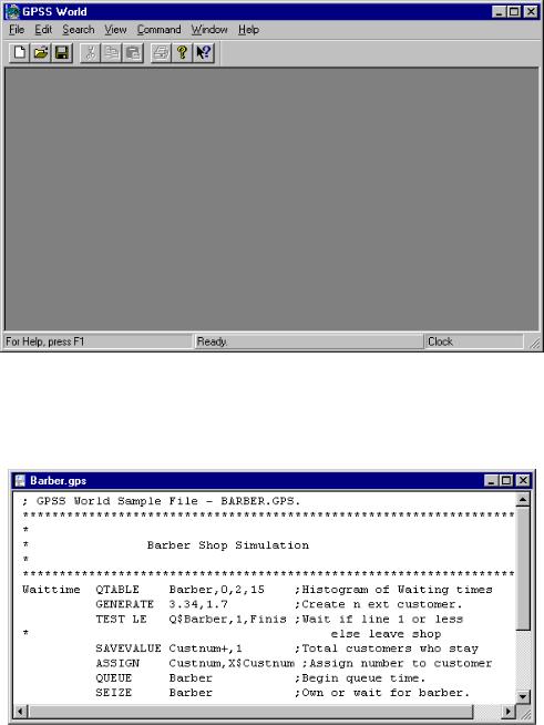
Figure 5—1. The Main Window
Figure 5—2. The Model Text Window
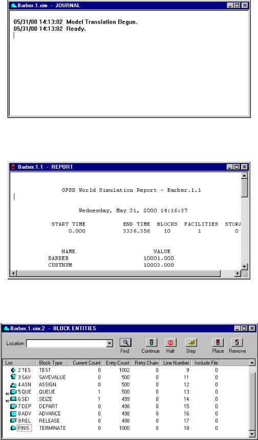
Figure 5—3. The Simulation Journal Window
Figure 5—4. The Report Window
Figure 5—5. Details View of the Blocks Window
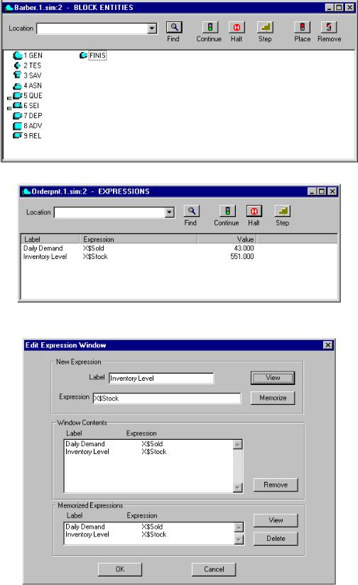
Figure 5—6. Non-detail View of the Blocks Window
Figure 5—7. The Expressions Window
Figure 5—8. The Edit Expressions Dialog
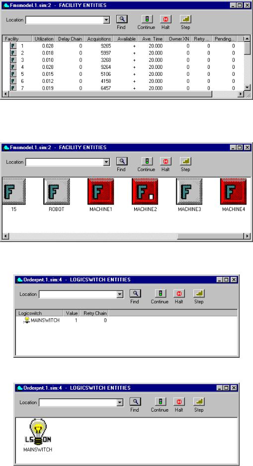
Figure 5—9. Detail View of the Facilities Window
Figure 5—10. Nondetail View of the Facilities Window
Figure 5—11. Detail View of the Logicswitches Window
Figure 5—12. Nondetail View of the Logicswitches Window
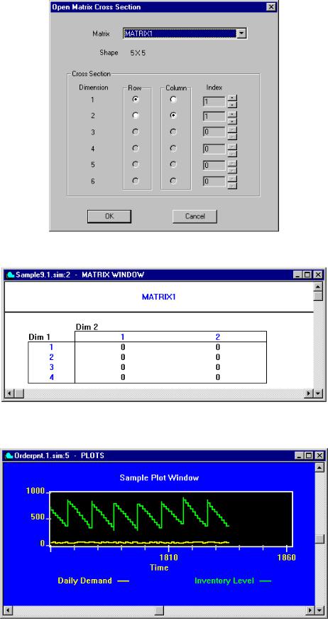
Figure 5—13. The Matrix Cross Section Dialog
Figure 5—14. The Matrix Window
Figure 5—15. The Plot Window
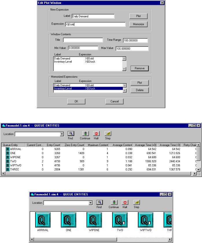
Figure 5—16. The Edit Plot Dialog
Figure 5—17. Detail View of the QueuesWindow
Figure 5—18. Nondetail View of the QueuesWindow
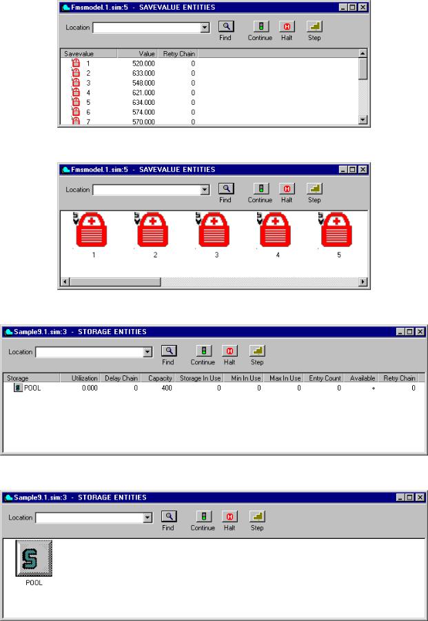
Figure 5—19. Detail View of the SavevaluesWindow
Figure 5—20. Nondetail View of the SavevaluessWindow
Figure 5—21. Detail View of the Storages Window
Figure 5—22. Nondetail View of the Storages Window