

In all records, except the last we have explicitly defined the tubing lengths, which are a little longer than the cell diameter of 100m, since the well path is partly diagonal to the grid. Since the distances have been defined, the rest can be defaulted.
In the last record, we are starting on the well segment which is parallel to the x-axis, in grid cell (14, 2, 3). When Dist0 is defaulted, the “current” friction length is taken as the last known value (Dist1 from the record above). When Dist1 is defaulted, it is computed as:
First the cell diameters are computed. Since the well direction is X, the diameter is 100m. Then we have defined a range – with direction X and start cell (14, 2, 3), the end index 19 means I=19, such that the end cell becomes (19, 2, 3). The range is hence six cells, and the total length is 600m (6*100), which is added to the Dist0.
Amalgamated grids
When WFRICTNL is used, the only difference is that in all records after the first, the first item is the LGR-name. The rest of the items are as before. If a range is used it must not span more than one LGR.
16. Numerical Solution of the Flow Equations
The objective is to give a “birds eye view” of how the flow equations are solved, without going into too much details. For such a discussion, the actual flow equations are not needed – it suffices to look at a representative equation containing the necessary features. The model equation will be,
∂u |
= |
∂2u |
+ |
∂2u |
+ |
∂2u |
(25) |
|
∂t |
∂x 2 |
∂y 2 |
∂z 2 |
|||||
|
|
|
|
Using central differences for the spatial approximation and forward difference in time, the finite difference approximation to Equation (25) is,
uin,+j,1k −uin, j,k |
= |
ui+1, j,k −2ui, j,k +ui−1, j,k |
+ |
ui, j+1,k −2ui, j,k +ui, j−1,k |
+ |
ui, j,k +1 |
−2ui, j,k +ui, j,k −1 |
(26) |
∆t |
(∆x)2 |
(∆y)2 |
|
(∆z)2 |
||||
|
|
|
|
|
In Equation (26), superscripts have been used to denote the time step. However, no time step has been indicated on the right hand side of the equation.
If the right hand side is evaluated at time step n, then the equation can be solved explicitly for the solution uin,+j,1k , which makes finding the solution at time n+1 for all cells (i, j, k) easy.
On the other hand, if the right hand side is evaluated at time n+1, then all the terms except uin, j,k are
unknown, and the system defined by Equation (26) when i,j,k take all values must be solved all at once, which is probably not straightforward. We denote this an implicit formulation of the problem, with an implicit solution procedure.
From numerical analysis it is known that the implicit solution is much more stable than the explicit solution, and the time steps can be larger. So even if an implicit solution scheme is harder to implement than an explicit scheme, it is generally worth the effort. As an example of the benefit, a stable scheme means that it will be self-correcting. I.e., if the solution at one time step has become erroneous for some reason, then the numerical solution will approach the “correct” solution at subsequent time steps. An explicit scheme does not in general have this property, which means that once an error starts to develop, it will grow with time, so that the solution gets worse and worse.
Both explicit and implicit schemes have been used in reservoir simulation through the years, but explicit schemes are not widely used any more. The default scheme in Eclipse is the implicit scheme, but IMPES (see below) is available as an option.
85
From Equation (26) it is apparent that the cells that enter each calculation are given by the 7-point stencil. I.e. to compute u in cell (i, j, k), we need the values in cells (i±1, j, k), (i, j±1, k), and (i, j, k±1).
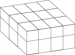
As an example, we will build the system structure for a grid with 4 cells in the x-direction, 3 in the y- direction, and 2 in the z-direction, i.e. nx=4, ny=3, nz=2. When we organize the system of equations we need to organize all the cells in one vector. We do this by the natural ordering, which is the same as the book order.
Then cell (1, 1, 1) will depend on (2,1,1), (1,2,1), and (1,1,2). But in the natural ordering that is equivalent to cell 1 depends on cells 2, 5 and 13.. In the same manner, cell (2,1,1) will depend on (1,1,1), (3,1,1), (2,2,1), and (2,1,2), i.e.: cell 2 depends on cells 1, 3, 6, and 14. (Ref. Figure 29)
|
2 |
|
|
3 |
|
4 |
|
1 |
|
|
|
|
|
||
|
|
|
|
8 |
|
||
|
|
|
|
7 |
|
||
|
|
|
6 |
|
|
||
|
5 |
|
|
|
|
||
|
|
|
|
|
|
||
|
|
|
|
|
11 |
12 |
|
|
|
|
|
|
10 |
||
|
|
9 |
|
|
|
||
|
|
|
|
|
|
||
13 |
|
|
|
|
|
|
|
|
|
|
|
|
|
|
|
|
17 |
|
|
|
|
|
|
|
21 |
|
|
|
22 |
23 |
24 |
|
|
|
|
|
|
||
|
|
|
|
|
|
|
Figure 29. Natural ordering of a 4 x 3 x 2 grid
Continuing this way we can draw a table (matrix) which depicts all the connections.
|
1 |
|
|
|
5 |
|
|
|
|
10 |
|
|
|
|
15 |
|
|
|
|
20 |
|
|
|
|
1 |
x |
x |
|
|
x |
|
|
|
|
|
|
|
x |
|
|
|
|
|
|
|
|
|
|
|
|
x |
x |
x |
|
|
x |
|
|
|
|
|
|
|
x |
|
|
|
|
|
|
|
|
|
|
|
|
x |
x |
x |
|
|
x |
|
|
|
|
|
|
|
x |
|
|
|
|
|
|
|
|
|
|
|
|
x |
x |
|
|
|
x |
|
|
|
|
|
|
|
x |
|
|
|
|
|
|
|
|
5 |
x |
|
|
|
x |
x |
|
|
x |
|
|
|
|
|
|
|
x |
|
|
|
|
|
|
|
|
|
x |
|
|
x |
x |
x |
|
|
x |
|
|
|
|
|
|
|
x |
|
|
|
|
|
|
|
|
|
x |
|
|
x |
x |
x |
|
|
x |
|
|
|
|
|
|
|
x |
|
|
|
|
|
|
|
|
|
x |
|
|
x |
x |
|
|
|
x |
|
|
|
|
|
|
|
x |
|
|
|
|
|
|
|
|
|
x |
|
|
|
x |
x |
|
|
|
|
|
|
|
|
|
|
x |
|
|
|
10 |
|
|
|
|
|
x |
|
|
x |
x |
x |
|
|
|
|
|
|
|
|
|
|
x |
|
|
|
|
|
|
|
|
|
x |
|
|
x |
x |
x |
|
|
|
|
|
|
|
|
|
|
x |
|
|
|
|
|
|
|
|
|
x |
|
|
x |
x |
|
|
|
|
|
|
|
|
|
|
|
x |
|
x |
|
|
|
|
|
|
|
|
|
|
|
x |
x |
|
|
x |
|
|
|
|
|
|
|
|
|
x |
|
|
|
|
|
|
|
|
|
|
x |
x |
x |
|
|
x |
|
|
|
|
|
|
15 |
|
|
x |
|
|
|
|
|
|
|
|
|
|
x |
x |
x |
|
|
x |
|
|
|
|
|
|
|
|
|
x |
|
|
|
|
|
|
|
|
|
|
x |
x |
|
|
|
x |
|
|
|
|
|
|
|
|
|
x |
|
|
|
|
|
|
|
x |
|
|
|
x |
x |
|
|
x |
|
|
|
|
|
|
|
|
|
x |
|
|
|
|
|
|
|
x |
|
|
x |
x |
x |
|
|
x |
|
|
|
|
|
|
|
|
|
x |
|
|
|
|
|
|
|
x |
|
|
x |
x |
x |
|
|
x |
|
20 |
|
|
|
|
|
|
|
x |
|
|
|
|
|
|
|
x |
|
|
x |
x |
|
|
|
x |
|
|
|
|
|
|
|
|
|
x |
|
|
|
|
|
|
|
x |
|
|
|
x |
x |
|
|
|
|
|
|
|
|
|
|
|
|
x |
|
|
|
|
|
|
|
x |
|
|
x |
x |
x |
|
|
|
|
|
|
|
|
|
|
|
|
x |
|
|
|
|
|
|
|
x |
|
|
x |
x |
x |
|
|
|
|
|
|
|
|
|
|
|
|
x |
|
|
|
|
|
|
|
x |
|
|
x |
x |
Figure 30. Coefficient matrix for a 4 x 3 x 2 grid (x means “nonzero element”)
86