

13. Fault modelling – Non-neighbour connections
It is clear from Figure 7 (or equivalent Figure 16 below) that one characteristic of faults is that, which grid cells are neighbours is different when a fault is present than not. The fault plane (in reality a volume) is typically an area of crushed rock, with poorer properties than the non-fault volume. To describe flow across a fault it is therefore necessary to define the possible flow paths, and the effective (reduced) fault permeability.
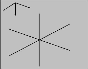
The 7-point stencil
The numerical approximation to the differential ∂∂fx in cell (I, J, K) was, using central differences,
∂f |
(I, J , K) ≈ |
f (I +1, |
J , K ) − f (I −1, |
J , K ) |
(24) |
|
∂x |
C(I +1, J , K ) −C(I −1, J , K ) |
|||||
|
|
|||||
where C(I, J, K) means the cell centre coordinate for cell (I, J, K), and f(I, J, K) means “f evaluated at the centre of cell (I, J, K)”.
J |
|
I |
|
K |
(I, J, K-1) |
||
|
|||
(I-1, J, K) |
(I, J-1, K) |
||
|
|
(I, J, K) |
|
|
|
(I+1, J, K) |
|
|
(I, J+1, K) |
|
|
|
|
(I, J, K+1) |
|
Figure 15. The 7-point stencil schematic
We see that ∂∂fx (I, J , K ) involves cells (I-1, J, K) and (I+1, J, K). In the same manner, ∂∂fy (I, J , K)
involves (I, J-1, K) and (I, J+1, K), and ∂∂fz (I, J , K ) involves (I, J, K-1) and (I, J. K+1).
In total, evaluating f and its differentials in all three directions in the cell (I, J, K) involves the cell itself and all the direct neighbours, (I±1, J, K), (I, J±1, K), (I, J, K±1), but not any diagonal neighbours. This computational scheme is called the 7-point stencil, and is shown schematically in Figure 15. The 7-point stencil is the basic computational molecule for Eclipse. Other computational schemes exist, with greater accuracy obtained by involving more points. In these notes we study only the 7-point stencil.
For a cell (I, J, K), the six other cells in the computational molecules are called its (logical) neighbour cells.
The fault layout – non-neighbour connections
In Chapter 4 we saw that Eclipse converts input permeabilities to inter-block transmissibilities, which are the connectivity parameters that are actually used during computations. The inter-block transmissibilities are computed for all cell-pairs that are neighbours, as in the 7-point stencil. When the grid contains a fault, these concepts will however need some modification.
67
Layer |
(I, J) |
|
|
|
|
1 |
(I+1, J) |
1 |
2 |
|
2 |
3 |
|
3 |
4 |
|
4 |
|
X |
|
|
Z |
|
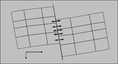
Figure 16. Sand to sand communication across a fault (vertical cross section)
In Figure 16 cell columns (I, J) and (I+1, J) are separated by a fault. A consequence of the fault is that cells (I, J, 1) and (I+1, J, 1) are no longer in contact with each other, and hence the transmissibility between these cells should be zero. On the other hand there is a direct flow path between cells (I, J, 3) and (I+1, J, 1), so the transmissibility between these two cells should be nonzero.
The arrows in Figure 16 show all possible flow paths between cells that are physical neighbours across the fault. Cells that are thus connected are said to be in sand-to-sand contact across the fault. The sand-to-sand contacts in the Figure are,
|
Upthrown side |
Downthrown side |
Layer |
2 |
1 |
|
3 |
1 |
|
3 |
2 |
|
4 |
2 |
|
4 |
3 |
During the initialisation phase, Eclipse will discover all sand-to-sand contacts, and modify the necessary transmissibilities accordingly. So in this case the affected transmissibilities that enter the 7- point stencil ( (I, J, K) to (I+1, J, K), for K=1,2,3,4) will be set to zero, and nonzero transmissibilities will be computed for all the cell pairs in the table.
Note that transmissibilities can be computed between any cell pair, not only cells which are logical neighbours. The most common case is when cells are in sand-to-sand contact, but there is no restriction at all regarding for which cell pairs nonzero transmissibilities can be defined.
Eclipse uses the term non-neighbour connection for such a case: The cells are not logical neighbours (i.e. their cell indices are not neighbours), but the transmissibility between the cells is non-zero (i.e. there is flow connectivity between the cells).
In the Figure 16 – example, cells (I, J, 2) and (I+1, J, 1) would be a non-neighbour connection, as would the cells (I, J, 4) and (I+1, J, 2).
We use the shorthand notation NNC-cells for cells which are connected by a non-neighbour connection.
Note: When defining NNC-cells across a fault, we are not restricted to cells which are in sand-to-sand contact, any cell pair can be an NNC. In reality fault flow is much more complex than just sand-to-sand flow, so it will often be necessary to define other NNCs than the ones Eclipse automatically constructs.
68
We could e.g. define flow from cell (I, J, 1) to (I+1, J, 1) in the Figure, even though these cells are not physical neighbours. Note also that this is an exceptional case, as these two cells are not non-neighbours, as they are neighbours in the sense of indexing. Flow between the cells (I, J, 2) and (I+1, J, 3) would however, be defined by an NNC. These are examples of more advanced modelling, and are outside the scope of these notes.
Fault transmissibility multipliers
It is often needed to modify (mainly reduce) the flow conductivity across the fault. As we have seen above, the fault flow is more complex than standard inter-cell flow, so modifying cell permeabilities is not flexible enough to control fault flow – we need to work with the transmissibilities directly. Eclipse offers several ways to do this, but we will only look at the method that is best suited for modifying transmissibilities between sand-to-sand contact cells. Eclipse computes initial values for all sand-to- sand transmissibilities honouring cell permeabilities and geometry (primarily the area of the shared surface). While doing this Eclipse also builds a table of which cells are in contact with which.
Again referring to Figure 16, where the flow across the fault is in the X-direction, the fault transmissibilities can be modified by the keyword MULTX. The keyword is most often used in the GRID section, but can also be used in EDIT or SCHEDULE sections (ref. Eclipse documentation). The easiest way to use MULTX is in combination with the EQUALS keyword. MULTX can be specified as many times as needed, and the syntax of each line is,
‘MULTX’ multiplier BOX /
The BOX is a cell box where the multipliers apply. When we specify a BOX for the MULTX keyword, the affected cell pairs are constructed by, for each cell in the box the cell’s X-face (i.e. the right hand face) is examined for sand-to-sand contact cells, and transmissibilities for all such contacts are modified. This is easier to envisage by an example. Still referring to Figure 16, assume now that the column denoted (I, J) is actually (6, 8). I.e. there is a fault between I=6 and I=7 for J=8. In practice faults usually are several cells long, so assume that the shown fault picture is valid for J=4,5,...,10.
To modify transmissibilities associated with layer 3 on the upthrown side, we would use the keyword,
EQUALS
‘MULTX’ 0.025 6 6 4 10 3 3 /
/
Now, the transmissibility between cells (6, J, 3) and (7, J, 1), and between cells (6, J, 3) and (7, J, 2) will be multiplied by 0.025, for all J = 4 – 10.
This is the really nice feature with MULTX compared to other, more manual methods to modify fault transmissibilities. MULTX acts on all sand-to-sand contact cell pairs emerging from the cells defined in the box, and we as users do not even need to know which cells are going to be affected – everything is taken care of automatically.
If we wanted to modify the whole fault in the same fashion, we would use,
EQUALS
‘MULTX’ 0.025 6 6 4 10 1 4 /
/
Note that we have included layer 1, even though layer 1 has no sand-to-sand contact across the fault (layer 1 on upthrown side – MULTX always acts in the direction of increasing I-index!), as Eclipse has no problems figuring out this itself, and arrive at the correct solution.
A commonly occurring situation is that the flow conductivity is dependent on the layers on both side of the fault. E.g. if layers 1 and 2 connect with the fault, we want the multiplier to be 0.1, but if layers 3 and 4 connect to the fault we want a multiplier of 0.02. The keyword would be,
69
EQUALS |
0.1 |
6 |
6 |
4 10 |
1 |
2 |
/ |
||
|
‘MULTX’ |
||||||||
|
‘MULTX’ |
0.02 |
6 |
6 |
4 10 |
3 |
4 |
/ |
|
/ |
|
|
|
|
|
|
|
|
|
and the resulting multipliers: |
|
|
|
|
|||||
|
|
|
|
|
|||||
|
|
Upthrown side |
Downthrown side |
Multiplier |
|||||
|
Layer |
|
2 |
|
|
1 |
|
|
0.1 |
|
|
|
3 |
|
|
1 |
|
|
0.02 |
|
|
|
3 |
|
|
2 |
|
|
0.02 |
|
|
|
4 |
|
|
2 |
|
|
0.02 |
|
|
|
4 |
|
|
3 |
|
|
0.02 |
The examples so far and Figure 16, have dealt with faults and multipliers in the X-direction, and MULTX applied to a group of cells and cells connected to this group in the direction of increasing I. The complete family of transmissibility multiplier keywords cover all cases. The syntax is identical, but the practical consequences are obviously different for the different cases.
MULTX |
Multipliers in +X direction (increasing I-index) |
MULTY |
Multipliers in +Y direction (increasing J-index) |
MULTZ |
Multipliers in +Z direction (increasing K-index) |
MULTX– |
Multipliers in –X direction (decreasing I-index) |
MULTY– |
Multipliers in –Y direction (decreasing J-index) |
MULTZ– |
Multipliers in –Z direction (decreasing K-index) |
The MULTZ and MULTZ– keywords are seldom used, and are not relevant for faults.
Note that if the negative index multipliers are used, they must be enabled by the keyword GRIDOPTS in the RUNSPEC section.
Multipliers are cumulative, i.e. if the same cells are modified several times, the effect will be cumulative. We demonstrate advanced use by an example. In the Figure 16 fault, we want the transmissibility multipliers to be 0.1 between 3 (upthrown) and 1 (downthrown), but 0.01 between 3 and 2. So a MULTX on layer 3 won’t work, since we want to treat 3 to 1 different than 3 to 2. For layers 2 to 1 we want a multiplier of 0.5, and connections from layer 4 should have no multiplier (i.e. multiplier = 1.0). The following combination of MULTX and MULTX– does it, (refer to the Figure while studying the example.)
EQUALS |
0.1 |
6 |
6 |
4 10 |
3 |
3 |
/ |
‘MULTX’ |
|||||||
‘MULTX-’ |
0.1 |
7 |
7 |
4 10 |
2 |
2 |
/ |
‘MULTX’ |
10.0 |
6 |
6 |
4 10 |
4 |
4 |
/ |
‘MULTX-’ |
0.1 |
7 |
7 |
4 10 |
3 |
3 |
/ |
/ |
|
|
|
|
|
|
|
Line 1: Multiplier set to 0.1 from layer 3, i.e. from (6, J, 3) to (7, J, 1) and (6, J, 3) to (7, J, 2)
Line 2: Multiplier set to 0.1 from layer 2 in cells I=7, and affecting cells with decreasing index, i.e. cells with I=6. So the cell pairs affected are (7, J, 2) to (6, J, 3) and (7, J, 2) to (6, J, 4). Since (6, J, 3) to (7, J, 2) already had a multiplier of 0.1 defined in line 1, this multiplier is now further multiplied by 0.1, and therefore the current value is 0.01 (as desired). The connection to layer 4 is wrong at this stage.
Line 3: Multiplier for cells (6, J, 4) to (7, J, 2) and (6, J, 4) to (7, J, 3) are set to 10. Since (6, J, 4) to (7, J, 2) was 0.1 it is now 1.0 (as desired)
Line 4: Fixes the connection (6, J, 4) to (7, J, 3), which was 10.0, now 1.0.
In real models it is generally not possible to model all faults as simple as e.g. “between cells I=6 and I=7 for J = 4 – 10.” To honour real fault geometry it is frequently necessary to let the fault trace be a
70
zig-zag line in the grid. In such cases the multipliers even for a single fault can become a long sequence of lines, where all combinations of MULTX, MULTX–, MULTY, and MULTY– occur. In some cases, editing and maintenance of the data file can be simplified by use of keywords FAULTS and MULTFLT, which are described below. Note that these keywords do nothing different than the “traditional” approach with the MULTX etc. keywords.
FAULTS – MULTFLT keywords (GRID section)
The FAULTS keyword is used to define the geometry of one or several named faults. Fault transmissibility multipliers can then later be defined by the MULTFLT keyword, which assigns a multiplier to the entire fault defined by the FAULTS keyword.
Note that the faults defined need not be real, complete faults. It is possible and recommended, to single out layers or groups of layers of whole or parts of a real fault, such that these can receive individual treatment later.
Syntax FAULTS:
Any number of lines, building the faults successively, each line terminated by a slash. Syntax of each line,
Fault name ix1 ix2 jy1 jy2 kz1 kz2 Face
Fault name |
Max 8 characters, used to identify fault |
ix1, ix2 |
Lower and upper I-index for the fault segment defined here |
jy1, jy2 |
Lower and upper J-index for the fault segment defined here |
kz1, kz2 |
Lower and upper K-index for the fault segment defined here |
Face |
Face of the fault, which is the same as the direction the transmissibility multiplier |
|
would be. Face X corresponds to using MULTX, and faces Y and Z similar. |
|
(Z seldom/never used). |
|
X–, Y–, Z– are also permitted (must set GRIDOPTS in RUNSPEC). |
There are some restrictions on the index bounds which are really obvious. If for example the face is X, then ix1 must be equal to ix2, etc. (purpose just to exclude impossible configurations).
Example
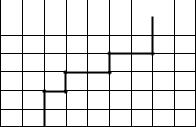
Assume we have a fault which looks as in Figure 17 (seen from above)
The model has 6 layers, and we want to define a transmissibility multiplier of 0.1 in the positive index direction from layers 1-3 across the fault, and a multiplier of 0.015 from layers 4-6 across the fault. We describe two different ways for defining the multipliers.
1 |
2 |
3 |
4 |
5 |
6 |
7 |
8 |
1
2
3
4
5
6
Figure 17. Example XY-view of fault.
1. Using multipliers
EQUALS |
value ix1 ix2 |
jy1 jy2 |
kz1 kz2 |
|
||||
--array |
/ |
|||||||
‘MULTX’ |
0.1 |
1 |
1 |
5 |
6 |
1 |
3 |
|
‘MULTY’ |
0.1 |
2 |
2 |
4 |
4 |
1 |
3 |
/ |
‘MULTX’ |
0.1 |
2 |
2 |
4 |
4 |
1 |
3 |
/ |
‘MULTY’ |
0.1 |
3 |
4 |
3 |
3 |
1 |
3 |
/ |
‘MULTX’ |
0.1 |
4 |
4 |
3 |
3 |
1 |
3 |
/ |
‘MULTY’ |
0.1 |
5 |
6 |
2 |
2 |
1 |
3 |
/ |
71