2. Using FAULTS and MULTFLT keywords

MULTFLT

-- f-name Multiplier Flt_top 0.1 / Flt_btm 0.015 /

/

We see that if this is a one-time job, the effort in setting up the fault and multiplier data is about the same in the two different approaches. The advantage with the latter method is seen if we want to change the multipliers to e.g. test sensitivities. Then we only have to change a single line in method 2, while more elaborate (and error prone) editing is required by method 1.

Defining a fault manually – the ADDZCORN keyword

As noted earlier, almost all grids of some complexity are constructed by dedicated software. This certainly includes fault definition and final representation of faults on the grid. Nevertheless, there are times when we would like to edit faults manually, either to do a minor fix that shouldn’t require a complete grid rebuild, or non-production grids, where we would like to construct generic faults without the need for the dedicated software. The means to do so in Eclipse are limited, and can seem cumbersome and complicated, but still the users should be aware of the possibilities that exist.

The keyword ADDZCORN is used to move individual corners in cells. It can be set to continuous mode, in which case adjacent corners are moved simultaneously, or cell corners can be moved without affecting neighbour corners.

Using ADDZCORN to move all corners of a cell (or box of cells) simultaneously

The data is given in three groups,

1.The distance to move corners, DZ

2.The box to move, ix1 ix2 jy1 jy2 kz1 kz2

In addition there is a flag for keeping the top or bottom layers unchanged,

72

Syntax: ADDZCORN can contain arbitrary many lines, each line with syntax,

DZ ix1 ix2 jy1 jy2 kz1 kz2 ix1A ix2A jy1A jy2A Top/Bottom-flag

Use of the continuity flags:

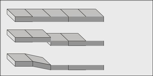
ix1A must be either the left hand boundary ix1, or the cell to the left of it (ix1-1). The value can be interpreted as, the first corner in the range to move. Hence, if ix1A is equal to ix1, cell ix1 is moved, but cell ix1-1 is left unchanged, whereby a discontinuity (fault) has been constructed. On the other hand, if ix1A is equal to ix1-1, then the right hand side of cell ix1-1 is moved (all associated corners are moved simultaneously), but the left hand edge of the cell is left unchanged. No discontinuity has hence been introduced. See Figure 18 for a visualisation of the use of the left hand (lower index) flag in the x-direction. The other flags act similar.

IX1A = IX1 = 5

IX1A = IX1-1 = 4

Figure 18. Example use of continuity flags in ADDZCORN, left hand x-direction

Example

We wish to move part of the grid downwards 20 m. The box to move is I = 5-10, J = 3-8. When moving the box, the left and right hand boundaries shall be discontinuous (fault) like in the middle example in Figure 18. The other two edges (J-direction) shall be continuous, like the lower example in the figure. The syntax is,

ADDZCORN

-- DZ ix1 ix2 jy1 jy2 kz1 kz2 ix1A ix2A jy1A jy2A TB-flag 20.0 5 10 3 8 1 6 5 10 2 9 /

/

Notes:

1.The continuity flags are only used when the box edge is continuous before the move. If a box edge prior to the move is discontinuous, like the middle example in Figure 18, then the box will be moved as discontinuous, and the rest of the grid left unchanged irrespective of the value of the continuity flag

2.All the indices ix1, ix2,..., jy1A must be within the grid index limits. I.e. if e.g. ix2 is at the right hand edge of the grid, it is an error to define ix2A = ix2+1. When the box extends to the edge of the grid the concept of continuity at the edge of the box becomes irrelevant anyway.

3.Normally all the layers are moved simultaneously. If only some layers are moved, the user must take care to avoid unintended overlaps or gaps after the move.

4.Note that the default values of the continuity flags imply continuity (no fault).

73