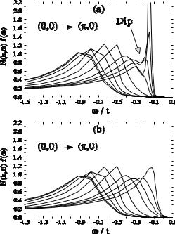
Fig. 3.31. Photoemission intensity N (k, ω)f (ω) (here N is the quasiparticle spectral function and f the Fermi function) for k = (kπ, 0), where k = 1, 7/8, 13/16, 3/4, 5/8, 1/2, 3/8, 1/4, 1/8, and 0. (a) in the superconducting state at T /Tc = 0.77. The narrow peaks at low binding energy decrease and vanish, and the binding energies of the broad humps increase in the sequence of k values. (b) In the normal state at T = 0.023t. Note that the broad humps are at the same positions as in the superconducting state.

shows that the gap in the scattering rate and the strong mass enhancement of the quasiparticles below Tc are decisive for the observability of this mode.

3.4.3 Collective Modes in Electronic Raman Scattering?

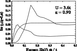
One can see from Fig. 3.30 that the resonance condition is approximately satisfied for ω0 = 2∆0 0.2t because then one enters the pair–breaking continuum, where Γ ω/2 near the antinode ka. Thus the mode frequency is about ω0 = 2∆0 for a damping Γ = ∆0, in agreement with the numerical results. In the weak–coupling limit, it has been shown that vertex corrections due to the d–wave pairing interaction together with electron–electron scattering lead to good agreement with the B1g Raman data on YBCO [151]. In Fig. 3.32, we show our strong-coupling results for the Raman response functions Im χγ (q = 0, ω), where γ is the vertex γ = t[cos(kx) − cos(ky )] and the vertex γ = −4t sin(kx) sin(ky ) for B1g and B2g symmetry, respectively. One

150 3 Results for High–Tc Cuprates: Doping Dependence

Fig. 3.32. Raman spectra Im χγ (q = 0, ω) for B1g symmetry at T = 0.023t (solid line) and T /Tc = 0.77 (dashed line), and Raman spectrum for B2g symmetry at T /Tc = 0.77 (dotted line). Tc = 0.022t.

can see that for B1g symmetry a gap and a pair–breaking threshold develop below Tc, with a threshold at about 0.15t (3/2)∆0 at T /Tc = 0.77 (see Fig. 3.31). Unfortunately, this means that the peak of the order parameter collective mode at ω0 2∆0 with a width ∆0 lies in the pair-breaking continuum. The question arises of whether or not the contribution of Im χf l to the B1g Raman spectrum is sizable, because the coupling strength proportional to NF /NF in (2.164) arising from particle–hole asymmetry is rather small. However, in the strong–coupling calculation, the coupling strength of

NF /NF , one obtains additional terms proportional to the self-energy components Re ξ(k, ω) and Im ξ(k, ω) which give relatively large contributions. In addition, one obtains a contribution from the imaginary part of the gap function, i.e. Im φ(k, ω).

Thus, the amplitude fluctuation mode of the d–wave gap derived in Sect. 2.3.3 couples only weakly to the charge fluctuations and yields a broad peak above the pair–breaking threshold in the B1g Raman spectrum. This peak may be, at least partially, responsible for the observed broadening above the pair–breaking peak because the coupling strength due to particle–hole asymmetry is enhanced by strong–coupling self-energy e ects. As already mentioned above previous work on collective modes in high–Tc superconductors has been restricted to weak-coupling and mean–field calculations. The FLEX approach that we have used here, is a self-consistent and conserving approximation scheme, which goes well beyond the mean–field approximation. The feedback e ect of the one-particle properties on the collective modes in the superconducting state is included self–consistently and the importance of the quasiparticle damping becomes clear. It is therefore a highly nontrivial and satisfactory result that the resonance in the spin susceptibility, the step–like edge in the quasiparticle scattering rate, and the dip features in the

ARPES and tunneling spectra can all be understood within one theory in a self-consistent fashion. The self-consistent calculation also yields a larger coupling strength of the d–wave amplitude mode to the charge density and a lower resonance frequency of the s–wave exciton–like mode of the order parameter, which makes it more likely that these modes might be observable in the B1g Raman scattering channel.

3.5 Consequences of a dx2−y2 –Wave Pseudogap

in Hole–Doped Cuprates

A few years ago, a normal–state pseudogap was inferred from inelastic neutron scattering (see [152] for a review), nuclear magnetic resonance [118], heat capacity [153], and resistivity [27] data on underdoped YBa2Cu3O7−δ and YBa2Cu4O8. Furthermore, angular–resolved photoemission spectroscopy measurements also indicated the presence of a dx2−y2 –wave gap well above Tc in the underdoped regime for many hole–doped cuprates [154]. Now, numerous experiments have established the fact that the underdoped cuprate superconductors exhibit a “pseudogap” behavior in both the spin and the charge degrees of freedom below a characteristic temperature T , which can be well above the superconducting transition temperature Tc. This has been discussed also in the Introduction. Furthermore, we have already demonstrated in Fig. 2.4 that the FLEX approach with the generalized Eliashberg equations yields the correct doping dependence T (x). However, the magnitude of the pseudogap shown in the inset of Fig. 2.4 is too small compared with experiment. Thus, we have extended our theory as described in detail in Sect. 2.2.

Many interpretations of the pseudogap have been advanced (see, for example the discussion in [155]); however, no consensus has been reached so far as to which of the various microscopic theories is the correct one. It has been shown by Williams et al. [155] that the specific–heat, susceptibility, and NMR data of many underdoped cuprates can be successfully modeled using a phenomenological normal–state pseudogap that has d–wave symmetry and an amplitude which is temperature–independent but increases upon lowering the doping level into the underdoped regime. The strong anisotropy of the pseudogap is also in accordance with ARPES experiments on underdoped Bi2Sr2CaCu2O8−δ (Bi2212) [154, 156]. This model yields a smooth evolution of the normal–state pseudogap into the superconducting gap, as has been found in STM experiments [10]. Also, measurements of the resistivity, Hall coe cient, and thermoelectric power can be reconciled with this model [27],[157]. In this section we follow this idea using the magnitude of the pseudogap Eg (see (2.67)) as an input into the generalized Eliashberg equations. The corresponding theory is described in Sect. 2.2. In the following we shall demonstrate the consequences of such a dx2−y2 -wave pseudogap for various

152 3 Results for High–Tc Cuprates: Doping Dependence

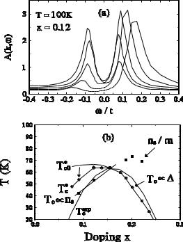
Fig. 3.33. (a) Results for the quasiparticle spectral function A(k, ω) versus ω for di erent k-vectors near the gap antinode: k = (0.14, 1), (0.16, 1), (0.17, 1), (0.19, 1), and (0.20, 1) (in units of π). The Fermi wave vector is ka = (0.18, 1)π. (b) Doping dependence of Tc and Tc obtained using a dispersion relation ˜(k) in accordance

with ARPES data. Tc is reduced from Tc0 (without pseudogap) to smaller values. For clarity, Tcexp(x) and ns (0)/m are also displayed. Tc0 refers to a mean–field

transition not taking the pseudogap in the tight–binding energy dispersion into account.

physical quantities, calculated self–consistently, of course. However, the origin of the pseudogap is still unknown.

3.5.1 Elementary Excitations and the Phase Diagram

As mentioned in Chap. 2, we obtain the right doping dependence of the (weak–) pseudogap temperature T ; however, the calculated magnitude of the pseudogap is too small in comparison with experiment. In general, the magnitude of this pseudogap should also influence the mean–field transition temperature Tc and thus the temperature range where preformed Cooper pairs are formed, because fewer holes (or electrons) can pair if fewer states at the Fermi level are present. In order to investigate this question in detail, we have performed calculations with an appropriate energy dispersion ˜(k) which

exhibits, in accordance with recent photoemission data, d–wave symmetry. Furthermore, we have chosen ˜(k) to be doping–dependent in accordance with [16, 17, 155, 158, 159].

In Fig. 3.33a, we present results for the spectral density A(k, ω) calculated within our FLEX theory in the underdoped regime from the Green’s function G(k, ω) [35]. We have used the Fermi surface observed by Marshall et al.

[159] and a dispersion ˜(k) = 2(k) + ∆2(k), including for k (π, 0) the pseudogap structure [35], as an input. The results show the interplay of the pseudogap and superconducting gap and the di erent features for underdoped and overdoped superconductors, and should be compared with SIN tunneling experiments and with ARPES data [159]. Of course, ARPES can measure only occupied states, i.e. the spectral density for ω < 0. As an example, we show in Fig. 3.33a our calculated spectral function for a doping concentration of x = 0.12 at T = 100 K, where the magnitude of the pseudogap is 0.1t = 25 meV. One can see that the spectral function does not cross the Fermi level (ω = 0). This has consequences for the Cooper pairing.

In Fig. 3.33b, we present the corresponding results for the phase diagram and for Tc (x) and Tc(x), obtained by using as an input dispersions ˜(k) which are, for underdoped cuprates, in accordance with recent angular–dependent photoemission results. As expected, if for k (π, 0), where pairing is most favorable, we take proper account of the observed pseudogaps [159], we obtain smaller values for Tc and Tc and for (Tc −Tc) as well (Tc0 is equivalent to Tc without a pseudogap in Fig. 2.4). The latter result signals that the pseudogap decreases the reduction of Tc → Tc due to Cooper pair phase fluctuations [160]. Thus we conclude that even if the reason for the pseudogap forming below T is unrelated to superconductivity, it will indeed influence Tc and Tc. Both temperatures are renormalized to smaller values owing to a reduced density of states at the Fermi level available for Cooperpairing. Also, the region where preformed pairs occur, Tc < T < Tc , is reduced.

Now we present results for the dynamical spin susceptibility, the NMR spin–lattice relaxation rate 1/T1T , and the Knight shift, obtained by solving the generalized Eliashberg equations with inclusion of the pseudogap using the extended FLEX approximation. We have again assumed that the pseudogap φc(k) has the simple form of a BCS–like d–wave gap, i.e. φc(k) ≡ ∆c(k) = Eg (cos kx − cos ky ), derived in Sect. 2.2.1. Furthermore, we have employed a tight–binding band (k) with first– and second–nearest– neighbor hopping (t = −0.45t), an e ective on–site repulsion U (q) having a maximum U = 3.6t at q = Q (t denotes the nearest–neighbor hopping energy), and a doping concentration x = 0.09.

Instead of solving the full set of equations (2.51)–(2.67), we have approximated these equations here by the simpler form which they acquire at the hot spots where the nesting condition 2 = − 1 is satisfied. This seems to be a reasonable approximation because these distinct points on the Fermi line yield the dominant contribution to the right–hand side of (2.51): first, the

154 3 Results for High–Tc Cuprates: Doping Dependence

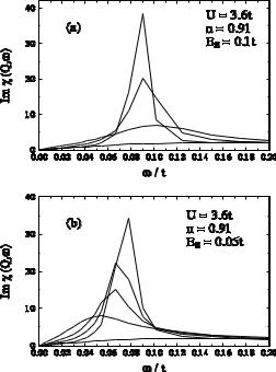
Fig. 3.34. Spectral density of spin susceptibility, Im χs(Q, ω) (where Q = (π, π)), versus ω in the underdoped regime. (a) The amplitude of the pseudogap taken as Eg = 0.1t and calculated for temperatures T = 0.1, 0.04, 0.025, and 0.02t (rising peaks in this sequence). (b) Comparison with results for Eg = 0.05t and T = 0.1, 0.025t, 0.021, 0.020, and 0.019t, the latter three temperatures corrseponding to the superconducting state (rising peaks in this sequence).

denominator of Gij (k ) becomes small, and second, the interaction Ps(k −k ) for scattering of quasiparticles from one hot spot to the other becomes large because k−k is of the order of Q = (−π, π) (see Fig. 2.8). This treatment of the d–wave pseudogap is somewhat similar to that of the CDW state in the work of Rice and Scott [161], although in our case the hot spots do not exactly coincide with the saddle points at (0, π) and (π, 0) (see Fig. 2.8). Hlubina and Rice [162] have shown that in the case of the resistivity, it is important not to restrict consideration to the hot spots, since a proper average over the whole Fermi surface can lead to di erent results. However, we would like to point out that we have performed our integrations over the whole Brillouin zone. For the pseudogap channel, we have approximated the Green’s functions using the form that they obey at the hot spots. This approximation is di erent in spirit from considering only the hot spots. All scattering processes due to spin fluctuations at all momentum points are taken into account. In addition, we have made this approximation only in the calculation of the self–energies

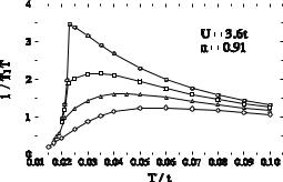
Fig. 3.35. The spin–lattice relaxation rate divided by T , 1/T1T , versus T , for amplitudes of the pseudogap Eg = 0 (dashed line) and Eg = 0.05, 0.075 and 0.1t (solid lines from top to bottom). The parameters are J(Q) = U = 3.6t (t is the next–nearest–neighbor hopping energy), and band filling n = 0.91 for an YBCO– like band, i.e. a doping concentration of x = 0.09. The superconducting transition temperatures are Tc = 0.023, 0.022, 0.021, and 0.0155t (from top to bottom).

and used these results for the calculation of the resistivity, which includes a full momentum average.

First, we consider the NMR and neutron scattering intensity in the underdoped regime, which we calculated from the spectral density of the dynamical spin susceptibility, Im χs(q, ω). This function has a broad peak as a function of q which is centered at Q = (π, π), and it exhibits a peak as a function of ω at the antiparamagnon energy ωsf . The slope of this function at ω = 0 first increases with decreasing T down to a crossover temperature, i.e. the pseudogap temperature T , and then it decreases with further decrease of T (see Fig. 3.34). At the same time, the peak at ωs Eg narrows and increases with decreasing T . The suppression of spectral weight is accompanied by a peak at higher energies, which resembles the resonance peak below Tc. Indeed, Dai et al. have observed a resonance-like peak in the underdoped regime of YBCO in the normal state [69]. However, this peak in Im χ(Q, ω) is not the resonance peak, since it has properties di erent from those seen in experiment (see footnote 5 in Sect. 3.2.1). This peak also does not follow from an ω–dependent gap and fulfills no resonance condition. The true resonance peak is a result of the feedback e ect of superconductivity, while the peak in the normal state is due to the pseudogap.

In Fig. 3.35, we have plotted the corresponding nuclear spin–lattice relaxation rate divided by T , 1/T1T , versus T . One can recognize that this quantity first increases with decreasing T , acquires a maximum at about the crossover temperature T , and then decreases rapidly as T tends to Tc. This behavior is plausible in view of the behavior of Im χs(Q, ω), because 1/T1T is essentially given by the slope of this function at ω = 0. The occurrence of a maximum of 1/T1T is in agreement with the NMR data in the underdoped

156 3 Results for High–Tc Cuprates: Doping Dependence

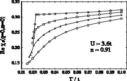
Fig. 3.36. The static, uniform spin susceptibility χs(q = 0, ω = 0), which is proportional to the Knight shift, versus T for pseudogap amplitudes Eg = 0, 0.05, 0.075, and 0.1t (curves in this sequence from top to bottom). The parameters are the same as in Fig. 3.35.

regime (see [163] for a review, and also [164]). In the overdoped regime of the cuprates, 1/T1T increases monotonically with decreasing T (again, see [163] for a review, and also [164]).

The temperature behavior of Im χs(Q, ω) is also in agreement with the temperature dependence of the neutron scattering intensity at a fixed small energy ω. This neutron scattering intensity first increases with decreasing T up to a maximum at about T and then decreases [152]. This behavior has been interpreted as a signature of the opening of a spin pseudogap in the spin excitation spectrum [152].

In Fig. 3.35, we also show 1/T1T for three di erent values of the amplitude Eg of the pseudogap in (2.67): Eg = 0.1t, 0.075t, and 0.05t. One can recognize that for this sequence of Eg values the position of the maximum at T decreases from about T = 0.06t to 0.045t and then to 0.035t, and that Tc (where the curve drops downwards) increases from about Tc = 0.0155 to 0.0206 and then to 0.0223. For Eg = 0, 1/T1T increases monotonically with decreasing T down to Tc0 0.023t. The decrease of Tc and the increase of T with increasing gap amplitude Eg are in qualitative agreement with the phase diagram of the Knight shift, magnetic susceptibility, and resistivity data in the underdoped regime [12, 165]. Here we assume implicitly that Eg increases as the doping away from half-filling, x = 1 − n, decreases.

The static, uniform spin susceptibility is proportional to χs(q = 0, ω = 0) = [1 − J(q = 0)χ0]−1χ0(q = 0, ω = 0). In Fig. 3.36, we have plotted our results for χs(0, 0) versus T for Eg = 0.1, 0.075 and 0.05t, and Eg = 0. One can see that χs decreases with decreasing T , and that the overall reduction down to Tc increases with increasing gap amplitude Eg in qualitative agreement with the fits of the NMR Knight shift data [165]. Here it should be pointed out that in our strong–coupling calculation, the pseudogap in (2.67) is reduced by Re Z and is smeared out by the quasiparticle damping ωIm Z.

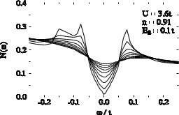
Fig. 3.37. Density of states N (ω) in the underdoped regime versus ω for U (Q) = U = 3.6t, band filling n = 0.91, size of the pseudogap Eg = 0.1t, and temperatures T = 0.1, 0.09, . . . , 0.02t (curves in this sequence from top to bottom). Only below Tc does the coherence peak develop.

The decrease of χs(0, 0), or χ0(0, 0), for decreasing T is plausible because χ0(0, 0) is approximately given by the BCS expression

where the density of states N (ω) is shown in Fig. 3.37 for Eg = 0.1t. One can see that N (ω) exhibits a typical d–wave gap, where N (ω) is linear in ω for ω < Eg . For decreasing T , N (0) decreases rapidly and therefore χ0 decreases with T .

Let us now come back to the spin–lattice relaxation rate. We have continued our calculation into the superconducting state somewhat below Tc. One can see from Fig. 3.35 that with decreasing T , the curve for 1/T1T exhibits a sharp downturn at Tc for Eg = 0, while the decrease of 1/T1T at Tc becomes slower and more continuous for increasing Eg . Similar results are obtained for χs, as shown in Fig. 3.36: the drop below Tc is abrupt for Eg = 0, while the decrease with T at Tc becomes slower and more continuous for increasing Eg . These results agree qualitatively with the spin–lattice relaxation rate and Knight shift data in the overdoped (corresponding to Eg = 0) and underdoped (corresponding to Eg > 0) regimes [164, 165]. For example, the experimental curves for 1/T1T in YBa2Cu3O7 and YBa2Cu3O6.52 [164] have a shape qualitatively similar to our curves for Eg = 0 and Eg > 0, respectively, in Figs. 3.35 and 3.36. The data in YBa2Cu4O8 etc. [165] are qualitatively similar to our results for Eg > 0 in Fig. 3.36.

To briefly summarize, the extension of the generalized Eliashberg equations by the inclusion of a dx2−y2 –wave pseudogap yields fair agreement with the spectral density, spin susceptibility, NMR spin–lattice relaxation rates, and Knight shift data. In particular, a peak in Im χ(Q, ω) develops (which resembles the resonance peak below Tc) as has been observed experimentally.