If c(t ) is small, cos c(t ) ≈ 1 and sin c (t ) ≈ c (t ), and (11.38) is simplified into form

When the modulating signal is sinusoidal c(t ) = 2p M cos (2p f m t ), we obtain

A (t ) ≈ A 0 {cos (2p f 0 t ) − p M sin [2p ( f 0 + f m ) t ] − pM sin [2p( f 0 − f m ) t ]} (11.40)

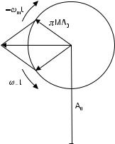
Equation (11.40) shows that the spectrum of a PM signal contains frequencies f 0 , f 0 + f m , and f 0 − f m , as an AM signal does, but now the phases of these components are different. Figure 11.22 represents a phasor diagram of the PM signal.

11.3.2 Digital Modulation

An analog signal, such as a voice signal in the form of an audio-frequency electric signal, can be transformed into a digital form by sampling it frequently

Figure 11.22 Phasor presentation of a PM signal.

298 Radio Engineering for Wireless Communication and Sensor Applications

enough. A digital signal may be binary, that is, containing only symbols 0 and 1, or m -ary, containing m different levels or states. The digital modulation has many advantages over the analog modulation; the total use of spectrum is effective, immunity to interference is good, frequency reuse is effective, TDM is easily realized, and it allows the use of encryption for privacy.

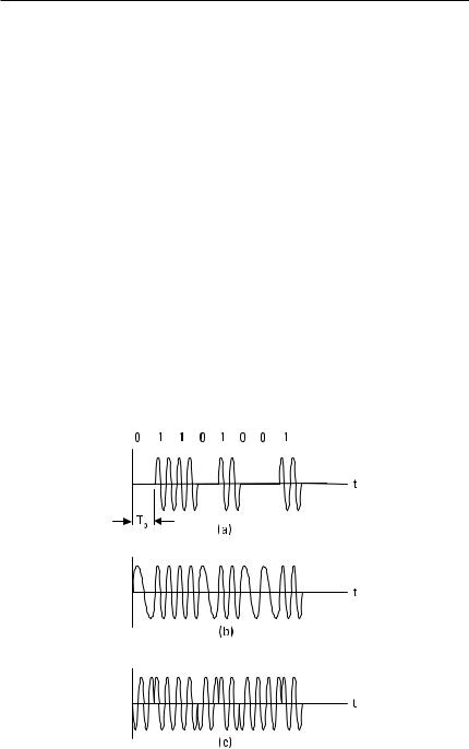
The basic digital modulation methods are amplitude-shift keying (ASK), frequency-shift keying (FSK), and phase-shift keying (PSK). Figure 11.23 shows the waveforms of binary ASK, FSK, and PSK signals when a symbol chain 01101001 is transmitted. In ASK, the maximum amplitude corresponds to symbol 1 and a zero amplitude corresponds to symbol 0. In FSK, the symbols are presented by signals with frequencies f 1 and f 2 . In PSK, signals corresponding to symbols 1 and 0 have a phase difference of 180°. While analog FM and PM signals closely resemble each other, FSK and PSK signals are easily distinguishable.

In digital modulation, rapid waveform changes occur and thus the power spectrum of a digitally modulated signal is broad. Figure 11.24 shows the spectra of a binary baseband signal consisting of rectangular pulses and a PSK signal modulated with it. The envelopes of the spectra have the shape of a sinc function. The width between the first nulls of the PSK spectrum is twice the bit rate 1/Tb , where Tb is the symbol period. In practice, the signal is filtered and the spectrum is narrower.

Figure 11.23 Waveforms of digitally modulated signals: (a) ASK, (b) FSK, and (c) PSK.

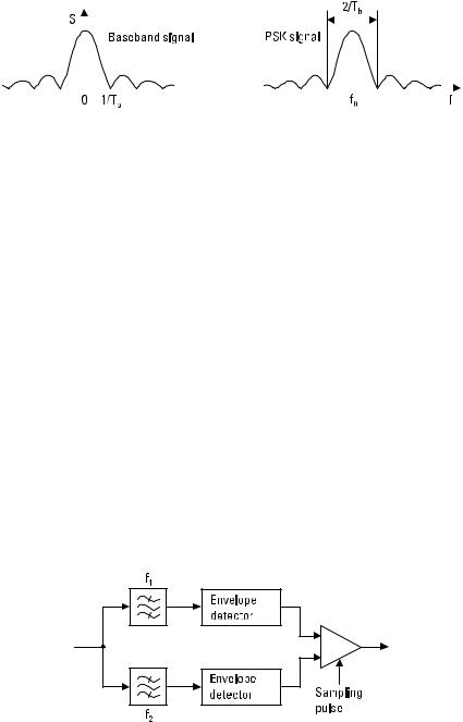
Figure 11.24 Spectra of a digital baseband signal and a PSK signal modulated with it.

In a binary modulation each symbol contains one bit of information. In a modulation scheme having 2m different states each symbol contains m bits. Then it is possible to transmit more information in a given bandwidth or to use a narrower band to transmit a given signal having a given bit rate. A four-state FSK (4FSK), four-state PSK (4PSK or QPSK), and eight-state PSK

(8PSK) are examples of modulation methods that save spectrum compared to the binary methods. In a digital QAM, both the amplitude and phase get several discrete values and the number of states may be 16, 64, or even higher. Therefore QAM is used in high-capacity links requiring effective use of the spectrum.

11.3.2.1 FSK

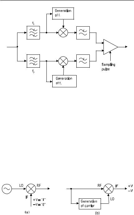
FSK can be realized by frequency modulating an oscillator or by switching between two oscillators operating at two different frequencies. The receiver may consist of two bandpass filters tuned for the frequencies f 1 and f 2 , and followed by envelope detectors. Decision between symbols 1 and 0 is made based on the output voltage of each detector. Such an FSK demodulator, presented in Figure 11.25, is said to be noncoherent.

A coherent demodulator, shown in Figure 11.26, provides a smaller bit error rate (BER). In the receiver, the frequencies f 1 and f 2 are regenerated, and their phases are synchronized with the incoming signal. The output

Figure 11.25 A noncoherent FSK demodulator.

300 Radio Engineering for Wireless Communication and Sensor Applications

Figure 11.26 A coherent FSK demodulator.

voltage of a phase detector (a double-balanced mixer) is proportional to the phase difference of these two signals. After filtering, the amplitudes are compared at the sampling time, and a decision is made between 1 and 0.

Minimum-shift keying (MSK) is a special case of FSK having the smallest separation of frequencies f 1 and f 2 so that the correlation between the symbols corresponding to 1 and 0 is zero. For MSK, the difference between f 1 and f 2 is half of the bit rate.

11.3.2.2 PSK

PSK can be realized by switching between two oscillators that have the same frequency but opposite phase, or with a double-balanced mixer, as shown in Figure 11.27(a). The double-balanced mixer acts as a polarity-reversing switch: When the sign of the voltage fed into the IF port changes, the phase of the carrier output from the RF port changes 180°. Demodulation takes

Figure 11.27 PSK: (a) modulation and (b) demodulation with a double-balanced mixer.

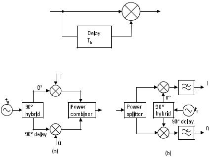
place in a reversed order, as in Figure 11.27(b). The carrier is regenerated in the receiver and fed into the LO port. The double-balanced mixer acts as a phase detector, and therefore the voltage from the IF port is either positive (+V = ‘‘1’’) or negative (−V = ‘‘0’’).

It may be difficult to get a phase synchronism between the carrier and the local oscillator during a period of only a few symbols. This difficulty can be avoided, and it is not necessary to generate the carrier in the receiver, if the phase of successive symbols is compared. Figure 11.28 shows such a differential PSK (DPSK) demodulator, where the signal is compared in a phase detector with the signal delayed by one symbol period Tb .

In quadriphase-shift keying (QPSK), the phase has four possible values, and each symbol corresponds to two bits: phase p/4 corresponds to 10, 3p /4 corresponds to 00, 5p/4 corresponds to 01, and 7p/4 corresponds to 11. A QPSK signal can be generated using the circuitry shown in Figure 11.29(a). The first bit of the pair is fed to the mixer of the upper branch (I = in-phase), and the second bit of the pair to the mixer of the lower branch (Q = quadrature phase). In the demodulator, shown in Figure 11.29(b), the carrier is regenerated and the phase detectors provide output voltages proportional to the bits.

Figure 11.28 A DPSK demodulator.

Figure 11.29 QPSK: (a) modulation and (b) demodulation.

302 Radio Engineering for Wireless Communication and Sensor Applications

11.3.2.3 QAM

The circuits in Figure 11.29 are also called an IQ-modulator and an IQdemodulator. They may be used to generate and detect digital QAM signals. For example, a 16QAM signal may be produced as a sum of a four-level I-signal and a four-level Q-signal. Figure 11.30 shows the constellation of the 16QAM signal on the IQ-diagram. Each point of the constellation presents one symbol now containing 4 bits. The distance of a point from the origin is proportional to the amplitude of the modulated carrier, and the angle between the positive I-axis and the direction of the point from the origin is analogous to the phase of the signal.

11.3.2.4 Comparison of Digital Modulation Methods

An ideal modulation method uses the radio spectrum efficiently, is robust against noise, interference, and fading, and can be realized with low-cost and power-efficient circuitry. However, these requirements are partly contradictory, and some tradeoffs have to be made to optimize the overall system performance.

Binary ASK, FSK, and PSK signals can be generated with simple circuits. Because ASK and FSK signals can be demodulated incoherently with an envelope detector, these receivers can also be made simple and inexpensive. Coherent detection of ASK and FSK requires more complex circuits but provides a lower BER. PSK has the lowest BER but requires generation of a synchronized carrier in the receiver.

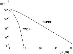
Figure 11.31 shows how the bit error rate of a PSK system depends on the S /N in an ideal AWGN channel and in a Rayleigh channel. In the AWGN channel, white noise is the only nonideality. An S /N of only about 7 dB is needed to achieve a BER of 10−3. Coherent FSK needs 3 dB higher

Figure 11.30 Constellation of 16QAM.