44 Radio Engineering for Wireless Communication and Sensor Applications

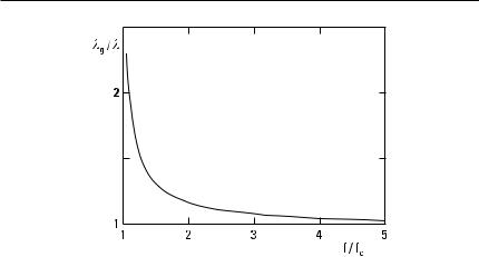
Figure 3.3 Wavelength of TE and TM waves above the cutoff frequency.

which is larger than the speed v of a plane wave in the same material as the insulator of the line. The propagation velocity of energy or the group velocity

is smaller than the speed of the plane wave in this material. Thus, the propagation velocity of TE and TM waves depends on frequency, and waveguides carrying these modes are dispersive.

3.4 Rectangular Waveguide

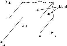
Both TE and TM wave modes may propagate in the rectangular waveguide shown in Figure 3.4. The longitudinal electric field of a TE mode is zero, Ez = 0, while for a TM mode the longitudinal magnetic field is zero, Hz = 0.

3.4.1 TE Wave Modes in Rectangular Waveguide

Let us assume that the solution of the longitudinal magnetic field has a form of

Figure 3.4 Rectangular waveguide.

where A is an arbitrary amplitude constant. By introducing the field of (3.34) to the equation of the TE wave mode, (3.24), we note that the differential equation is fulfilled if

46 Radio Engineering for Wireless Communication and Sensor Applications

From the boundary conditions for the fields in a metal waveguide it follows that the transverse magnetic field cannot have a normal component at the boundary, that is, n ? H = 0. It follows from (3.7) and (3.8) that

∂Hz /∂x = 0, when x = 0 or a , and ∂Hz /∂y = 0, when y = 0 or b.

Also, the tangential component of the electric field must vanish at the

boundary or n × E = 0: Ex (x , 0) = 0, Ex (x , b ) = 0, Ey (0, y ) = 0, Ey (a, y ) = 0.

It results from these boundary conditions that k 1 a = np and k 2 b = mp, where n = 0, 1, 2, . . . and m = 0, 1, 2, . . . , and therefore,

The cutoff wavelength and cutoff frequency are:

The subscripts n and m refer to the number of field maxima in the x and y directions, respectively.

In most applications, we use the fundamental mode TE10 having the lowest cutoff frequency:

In the case of an air-filled waveguide, we obtain f cTE 10 = c /(2a ). The cutoff wavelength is lc = 2a . If the waveguide width a is twice the height b, a =

2b , the TE20 and TE01 wave modes have a cutoff frequency of 2 f cTE 10 . The fields of the TE10 wave mode are solved from the Helmholtz

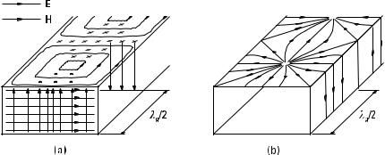
E0 is the maximum value of the electric field, which has only a y -component. All field components depend on time and the z -coordinate as exp ( jv t − gz ). Figure 3.5 illustrates the fields and the surface currents of the TE10 wave mode.

The wave impedance of the TE10 mode is

For example, at a frequency of 1.5f c , the wave impedance of an air-filled waveguide is 506V. The wave impedance depends on frequency and is characteristic for each wave mode.

The characteristic impedance Z 0 of a transmission line is the ratio of voltage and current in an infinitely long line or in a line terminated with a

Figure 3.5 (a) Fields and (b) surface currents of the TE10 wave mode in a rectangular waveguide at a given instant of time.

48 Radio Engineering for Wireless Communication and Sensor Applications

matched load having a wave propagating only in one direction. However, we cannot uniquely define the voltage and current of a waveguide as we can do for a two-conductor transmission line. Therefore, we may have many definitions for the characteristic impedance of a waveguide using any two of the following three quantities: power, voltage, current. The characteristic impedance can be calculated from the power propagating in the waveguide, Pp given in (3.53), and the voltage U, which is obtained by integrating the electric field in the middle of the waveguide from the upper wall to the lower wall, as

Note that the characteristic impedance of the TE10 wave mode depends on the height b, whereas the wave impedance of (3.50) does not. The characteristic impedance in (3.51) has been found to be the best definition in practice when problems concerning impedance matching to various loads are being solved.

The power propagating in a waveguide is obtained by integrating Poynting’s vector over the area of the cross section S :

S

The power propagating at the TE10 wave mode is

S

The finite conductivity of the metal, sm , causes loss in the walls of the waveguide. Also, the insulating material may have dielectric loss due to er″ and conduction loss due to sd . The attenuation constant can be given as

where P l is the power loss per unit length.

The power loss of conductors is calculated from the surface current density Js = n × H (n is a unit vector perpendicular to the surface) by integrating | Js |2R s /2 over the surface of the conductor. Although in the preceding analysis the fields of the waveguide are derived assuming the conductors to be ideal, this method is accurate enough if the losses are low. The surface resistance of a conductor is R s = √vm0 /(2sm ). The attenuation constant of conductor loss for the TE10 wave mode is obtained as

Close to the cutoff frequency, the attenuation is high, approaching infinite. If the dielectric material filling the waveguide has loss, the attenuation constant of dielectric loss is for all wave modes

The total attenuation constant is a = ac + ad .

The recommended frequency range for waveguides operating at the TE10 wave mode is about from 1.2 to 1.9 times the cutoff frequency f cTE 10 . The increase of attenuation sets the lower limit, whereas the excitation of higher-order modes sets the higher limit. Hence, we need a large number of waveguides to cover the whole microwave and millimeter-wave range. Standard waveguides that cover the 10 GHz to 100 GHz range are listed in Table 3.2. In most cases a = 2b. Figure 3.6 shows the theoretical attenuation of some standard waveguides made of copper. In practice, the attenuation is higher due to the surface roughness.

Example 3.1

Find the maximum power that can be fed to a WR-90 waveguide at 10 GHz. The maximum electric field that air can withstand without breakdown—the dielectric strength of air—is about 3 kV/mm.

Solution

The dimensions of the waveguide are a = 22.86 mm and b = 10.16 mm. From (3.50), the wave impedance of the TE10 wave mode at 10 GHz

(l = 30 mm) is Z TE 10 = 500V. By setting E0 = 3 kV/mm into (3.53), we find the maximum power to be 1.05 MW. Because the attenuation is about