

Fundamentals of Electromagnetic Fields |
17 |
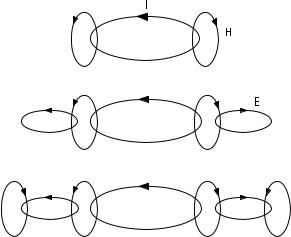
Figure 2.2 Electromagnetic wave produced by a current loop.
2.2 Fields in Media
In the above equations, the permittivity e and permeability m represent the properties of the medium. A medium is homogeneous if its properties are constant, independent of location. An isotropic medium has the same properties in all directions. The properties of a linear medium are independent on
field strength.
In a vacuum, e = e0 ≈ 8.8542 × 10⁻¹² F/m and m = m0 = 4p × 10−7 H/m. In other homogeneous media, e = er e0 and m = mr m 0 , where the dielectric constant er , that is, the relative permittivity, and the relative permeability, mr , depend on the structure of the material. For air we can take er = mr = 1 for most applications. In general, in a lossy medium, er or m r are complex, and in an anisotropic medium er or mr are tensors.
Let us consider a dielectric that has no freely moving charges. The electric field, however, causes polarization of the material, that is, the electric dipole moments tend to align along the field. The field induces a dipole moment into the atoms by disturbing the movement of electrons. The socalled polar molecules, such as the water molecule, have a stationary dipole moment, because the charge is distributed unevenly in the molecule.
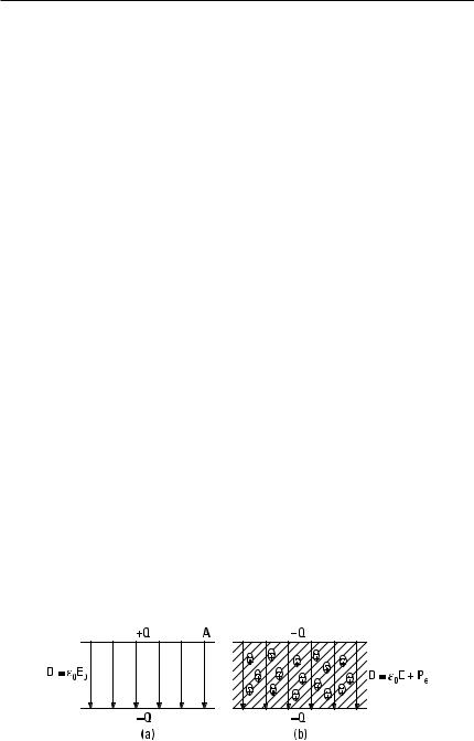
Electric polarization may be illustrated with a plate capacitor, the plates of which have an area of A and charges of +Q and −Q . If the fringing field lines are negligible, the electric flux density is D = Q /A . If there is vacuum (or air) between the plates, the electric field strength is E0 = D /e0 ; see
18 Radio Engineering for Wireless Communication and Sensor Applications
Figure 2.3(a). When a dielectric material is introduced between the plates, the dipole moments align along the field lines; see Figure 2.3(b). The flux density does not change if Q does not change, because the charge density in the dielectric is zero. However, the field strength decreases, because the field caused by the dipole moments cancels part of the original field. Therefore, the electric flux density may be written as
D = e 0 E + Pe |
(2.27) |
where Pe is a dipole moment per unit volume due to polarization. If a constant voltage is applied between the plates, the electric field strength stays constant, and the electric flux density and the charge of the plates increase when dielectric material is introduced between the plates. In a linear medium, the electric polarization depends linearly on the field strength
Pe = e 0 xe E |
(2.28) |
where xe is the electric susceptibility, which may be complex. Now |
|
D = e0 (1 + xe )E = eE |
(2.29) |
where |
|
e = e 0 (1 + xe ) = e 0 er = e0 (er′ − jer″ ) |
(2.30) |
is the complex permittivity. The imaginary part is due to loss in the medium; damping of the vibrating dipole moments causes heat, because the polar molecules cannot follow the changing electric flux due to friction.
The loss in a medium may also be due to conductivity of the material. In this case there are free charges in the material that are moved by the
Figure 2.3 Plate capacitor, which has as its insulator (a) vacuum, and (b) dielectric material that has electric dipole moments.

Fundamentals of Electromagnetic Fields |
19 |
electric field. When the conduction current density J = sE is introduced in Maxwell’s IV equation, one obtains
= × H = [s + jve0 (er′ − jer″)]E = jve0 Ser′ − jer″ − j ves 0 DE
(2.31)
which shows that damping due to polarization and damping due to conduction are indistinguishable without a measurement at several frequencies. Often s/(ve0 ) is included in er″. Loss of a medium is often characterized by the loss tangent
tan d = |
er″ + s/(ve0 ) |
|
(2.32) |
|
er′ |
||||
|
|
|||
which allows us to write (2.31) in form |
|
|||
= × H = jve0 er′(1 − j tan d ) E |
(2.33) |
|||
In case of magnetic materials, the situation is analogous: The magnetic field aligns magnetic dipole moments, that is, polarizes the material magnetically. The permeability can be divided into a real part m r′ and an imaginary part m r″; the latter causes magnetic loss.
The same medium may be considered as a dielectric at a very high frequency but a conductor at a low frequency. One may argue that a material is a dielectric if s/(ver′e0 ) < 1/100 and a conductor if s/(ver′e0 ) > 100. Table 2.1 shows conductivity, the real part of the dielectric constant, and the frequency at which the conduction current is equal to the displacement current for some media common in nature.
Table 2.1
Conductivity, Real Part of Dielectric Constant, and Frequency f T at Which the Conduction Current Is Equal to the Displacement Current of Some Materials
Material |
s [S/m] |
er′ |
f T [MHz] |
|
|
|
|
|
|
Sea water |
5 |
|
70 |
1300 |
Fresh water |
3 × 10⁻³ |
80 |
0.7 |
|
Moist soil |
10−2 |
|
30 |
6 |
Dry soil |
10−4 |
|
3 |
0.6 |
Ice |
10−5 |
. . . 10−4 |
3 |
0.06–0.6 |
20 Radio Engineering for Wireless Communication and Sensor Applications
2.3 Boundary Conditions
In electronics and radio engineering we often have electromagnetic problems where the properties of the medium change abruptly. We have to know the behavior of fields at such interfaces, that is, we have to know the boundary conditions. They can be deduced from Maxwell’s equations in integral form.
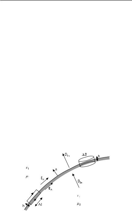
Let us consider a general interface between the two media presented in Figure 2.4. Medium 1 is characterized by e 1 and m 1 , and medium 2 by e 2 and m 2 . In the following, fields normal to the surface (of the interface) are denoted with subscript n and fields tangential to the surface with subscript t .
Let us consider a closed contour with dimensions Dl and h as shown in Figure 2.4. If h approaches 0, we obtain from Maxwell’s III equation, (2.24):
RE ? d l = E 1t Dl − E 2t Dl = −jv EB ? d S
G S
which approaches zero because as the area Dlh vanishes, the magnetic flux through the contour must also vanish. Therefore E1t = E2t , or
n × (E1 − E2 ) = 0 |
(2.34) |
Next we utilize Maxwell’s IV equation, (2.25)
Figure 2.4 Boundary between two media.
|
Fundamentals of Electromagnetic Fields |
21 |
||
R |
H ? d l = H1t Dl − H2t Dl = |
E |
( J + jvD) ? d S |
|
|
|
|
||
G |
|
S |
|
|
which approaches a value of Js Dl as h approaches zero, because when the area Dlh vanishes the electric flux through the contour must vanish, but a current remains due to the surface current density Js at the interface. Now we obtain
n × (H1 − H2 ) = Js |
(2.35) |
Next we consider a ‘‘pillbox,’’ a cylinder also shown in Figure 2.4. Its dimensions are height h and end surface area DS. Utilizing Maxwell’s I equation, (2.22), in the case where h approaches 0, we obtain
RD ? d S = D 2n DS − D1n DS = E rdV = rs DS
S V
where r s is the surface charge density at the interface. Now we obtain the following boundary condition:
n ? (D1 − D2 ) = n ? (e1 E1 − e2 E2 ) = r s |
(2.36) |
Similarly we can derive the following result for the magnetic flux density B (Maxwell’s II equation):
n ? (B1 − B2 ) = n ? (m1 H1 − m2 H2 ) = 0 |
(2.37) |
In case of an interface between two media, we obtain the following boundary conditions:
n × (E1 − E2 ) = 0 |
(2.38) |
|
n × (H1 |
− H2 ) = 0 |
(2.39) |
n ? (D1 |
− D2 ) = 0 |
(2.40) |
n ? (B1 − B2 ) = 0 |
(2.41) |
|
These equations state that the tangential components of E and H as well as the normal components of D and B are equal on both sides of the interface, that is, they are continuous across the interface.