

242 Radio Engineering for Wireless Communication and Sensor Applications
planar array, which consists of 16 microstrip antenna elements fed in phase and with equal amplitudes. This array is like the rectangular aperture antenna treated in Section 9.6. Many kinds of different patterns can be realized by choosing proper amplitudes and phases for the elements. Besides microstrip elements, an array may consist of many other types of elements such as dipoles, slots, or horns [9].
If there are electronically controlled phase shifters in the feed network of an array, the direction of the beam can be changed rapidly without rotating the antenna. This kind of electronic scanning is much faster than mechanical scanning. A phased array combined with digital signal processing may operate as an adaptive antenna. The pattern of an adaptive antenna changes according to the electromagnetic environment; for example, the beam of a base-station antenna may follow a moving user and a null may be formed in the direction of an interfering signal. An adaptive antenna may also partly correct the deterioration of its pattern, if one or more of its elements breaks down. Adaptive antennas are also called ‘‘smart’’ antennas.
9.11 Matching of Antennas
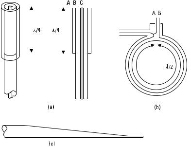
In principle, an antenna may be matched as any load impedance. However, some wire antennas, such as dipole and loop antennas, need a special attention if they are fed from an unsymmetrical line. For example, if a dipole antenna is connected directly to a coaxial line, currents will flow on the outer surface of the outer conductor. Then the outer conductor will radiate and the directional pattern will be distorted.
The radiation of the outer conductor can be prevented with a balun, a balanced-to-unbalanced transformer. The balun of Figure 9.33(a) has a short-circuited quarter-wave line outside the outer conductor. Thus, the impedance between A and B is large. Now, a symmetric load as a dipole antenna can be connected between A and C so that the outer conductor does not radiate. The balun of Figure 9.33(b) transforms the characteristic impedance of the coaxial line, Z 0 , to an impedance of 4Z 0 between A and B. In the balun of Figure 9.33(c) the coaxial line changes gradually to a parallel-wire line.
9.12 Link Between Two Antennas
Let us assume that a signal is transmitted from one antenna to another. The antennas are in free space and their separation r is large compared to the
|
|
|
|
|
|
|
|
Antennas |
243 |
||
|
|
|
|
|
|
|
|
|
|
|
|
|
|
|
|
|
|
|
|
|
|
|
|
|
|
|
|
|
|
|
|
|
|
|
|
|
|
|
|
|
|
|
|
|
|
|
|
|
|
|
|
|
|
|
|
|
|
|
|
|
|
|
|
|
|
|
|
|
|
|
|
|
|
|
|
|
|
|
|
|
|
|
|
|
|
|
|
|
|
|
|
|
|
|
|
Figure 9.33 Baluns: (a) a short-circuited sleeve of a length l /4 over a coaxial cable; (b) a loop of a length l /2 of a coaxial line; and (c) the outer conductor of a coaxial line changes gradually to a parallel-wire line.
distances obtained from (9.1). The main beams of the antennas are pointing toward each other and their polarizations are matched.
If the power accepted by the transmitting antenna, Pt , were transmitted isotropically, the power density at a distance of r would be
Sisot = |
Pt |
|
(9.58) |
|
4p r |
2 |
|||
|
|
The maximum power density produced by the transmitting antenna having a gain of Gt is
S = |
Gt Pt |
|
(9.59) |
||
4p r |
2 |
||||
|
|
||||
The corresponding electric field amplitude produced by the antenna is
E = √ |
2hS |
(9.60) |

244 Radio Engineering for Wireless Communication and Sensor Applications
The power available from the receiving antenna is its effective area A r times the power density of the incoming wave:
Pr = A r S |
(9.61) |
Using (9.4) and (9.59), this can be written as the Friis free-space equation:
Pr = Gt Gr S |
l |
D2 Pt |
(9.62) |
4p r |
where Gr is the gain of the receiving antenna.
In practice, many factors may reduce the power received, such as errors in the pointing of the antennas, polarization mismatch, loss due to the atmosphere, and fading due to multipath propagation. Losses due to impedance mismatches also have to be taken into account; generally, the power accepted by the transmitting antenna is smaller than the available power of the transmitter, and the power accepted by the receiver is smaller than the available power from the receiving antenna.
Example 9.3
What is the loss Pt /Pr at 12 GHz from a geostationary satellite at a distance of 40,000 km? Both the transmitting and receiving antennas have a diameter of D = 1m and an aperture efficiency of hap = 0.6.
Solution
The antennas have an effective area of A eff = hap pD 2/4 = 0.47 m2 and a gain of G = 4p A eff /l 2 = 9 500. The loss Pt /Pr = (4p r /Gl)2 = 4.5 × 10¹²,
in decibels 10 log (4.5 × 10¹² ) dB = 126.5 dB. Here, the attenuation of the atmosphere is not taken into account. During a clear weather, the atmospheric attenuation is about 0.3 dB at 12 GHz.
Example 9.4
How accurately the receiving antenna of the preceding example has to be pointed to the satellite, if the allowed maximum pointing loss is 0.5 dB? The satellite transmits two orthogonal, linearly polarized signals. How accurately must the tilt angle of the linearly polarized receiving antenna be adjusted if (a) the maximum loss due to polarization mismatch is 0.5 dB, and if (b) the maximum power coupled between the orthogonal channels is −30 dB?
Antennas |
245 |
Solution
The beamwidth of the receiving antenna is u 3dB ≈ 1.2l/D = 0.03 rad = 1.7°. The pattern level depends approximately quadratically on the angle
near the main beam maximum. Thus, the maximum allowed pointing error is (0.5/3)1/2 × 1.7°/2 = 0.35°. The antenna receives only the component of the incoming wave that has the same polarization as the antenna. (a) From 20 log (cos Dt ) = −0.5 we solve that an error of Dt = 19.3° in the tilt angle reduces the received power by 0.5 dB. (b) From 20 log (sin Dt) = −30 we solve that Dt = 1.8° gives a cross-polar discrimination of 30 dB. Thus, to avoid interference between the orthogonal channels, the error in the tilt angle should not be too large.
References
[1]Kraus, J. D., and R. J. Marhefka, Antennas for All Applications, 3rd ed., New York: McGraw-Hill, 2002.
[2]Lo, Y. T., and S. W. Lee, (eds.), Antenna Handbook: Theory, Applications, and Design,
New York: Van Nostrand Reinhold, 1988.
[3]Rudge, A. W., et al., (eds.), The Handbook of Antenna Design, Vol. 1, London, England: Peter Peregrinus, 1982.
[4]Rudge, A. W., et al., (eds.), The Handbook of Antenna Design, Vol. 2, London, England: Peter Peregrinus, 1983.
[5]Fujimoto, K., and J. R. James, (eds.), Mobile Antenna Systems Handbook, Norwood, MA: Artech House, 1994.
[6]Garg, P., et al., Microstrip Antenna Design Handbook, Norwood, MA: Artech House, 2001.
[7]Lee, K. F., and W. Chen, (eds.), Advances in Microstrip and Printed Antennas, New York: John Wiley & Sons, 1997.
[8]Chatterjee, R., Dielectric and Dielectric-Loaded Antennas, New York: John Wiley & Sons, 1985.
[9]Sehm, T., A. Lehto, and A. Ra¨isa¨nen, ‘‘A High-Gain 58-GHz Box-Horn Array Antenna with Suppressed Grating Lobes,’’ IEEE Trans. on Antennas and Propagation, Vol. 47, No. 7, 1999, pp. 1125–1130.