

120 Radio Engineering for Wireless Communication and Sensor Applications
application, typically 3 dB to 30 dB. The directivity describes the leakage to the isolated port and should be as large as possible; a good directivity may be 30 dB to 40 dB. The isolation between the input port and the isolated port is C + D in decibels.
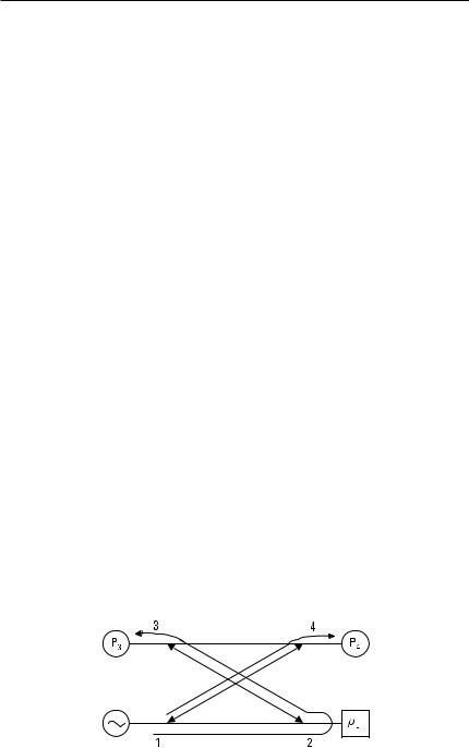
A directional coupler with a good directivity can discriminate between the waves propagating in opposite directions on a line. However, mismatches of the output loads may worsen the effective directivity. Let us consider the situation illustrated in Figure 6.6. A signal source is connected at port 1, an unknown load with a reflection coefficient of r L is connected at port 2, and matched power meters are connected to ports 3 and 4. In an ideal case the power meter readings are
P 3 = | rL |2 |
|
1 − |
1 |
|
1 |
P 1 and P 4 = |
1 |
P 1 |
|
S |
10C /10 D |
10C /10 |
10C /10 |
||||||
|
|
|
|
||||||
from which the magnitude of the reflection coefficient can be solved. If the directional coupler has a finite directivity, and the signal source and power meters are mismatched, several waves will disturb the measurement and cause errors. An accurate analysis is complicated since there will be multiple reflections between the mismatches. The analysis may be carried out using a flow graph. Approximate error limits may be calculated by taking only the first reflections into account. When summing up the waves propagated to the power meters via different paths, both the amplitudes and phases of the waves must be taken into consideration. Summing up the powers of individual waves is not correct.
6.1.3 Scattering Matrix of a Directional Coupler
Let us next derive the scattering matrix of an ideal directional coupler. Because ports 1 and 3 as well ports 2 and 4 are isolated from each other,
Figure 6.6 Measuring the magnitude of the reflection coefficient with a directional coupler.
Passive Transmission Line and Waveguide Devices |
121 |
S13 = S24 = 0. Let us assume that ports 1 and 2 are matched, or S11 = S22 = 0. Due to the reciprocity Sij = Sji . Thus, the scattering matrix is
|
0 |
S12 |
0 |
S14 |
4 |
|
|
[S ] = |
S12 |
0 |
S23 |
0 |
(6.10) |
||
0 |
S23 |
S33 |
S34 |
||||
|
|
||||||
|
3S14 |
0 |
S34 |
S44 |
|
The scattering matrix of a lossless circuit is unitary. From rows 1 and
4 we get S14 S44* = 0 and from rows 2 and 3 S23 S33* = 0. Because S14 and S23 are nonzero, parameters S33 and S44 must be zero, and ports 3 and 4
must be matched. From rows 1 and 3 and from rows 2 and 4 we get the following equations, respectively,
S12 S23* |
+ S14 S34* |
= 0 |
(6.11) |
S12 S14* |
+ S23 S34* |
= 0 |
(6.12) |
Because, for example | S12 S23* | = | S12 | | S23 | , (6.11) and (6.12) can be written as
| S12 | | S23 | = | S14 | | S34 | |
(6.13) |
| S12 | | S14 | = | S23 | | S34 | |
(6.14) |
By dividing the left side and right side of (6.13) with the corresponding
sides of (6.14), we get | S23 | / | S14 | = | S14 | / | S23 | , which means that | S14 | = | S23 | . Hence the coupling between ports 1 and 4 is equal to that
between ports 2 and 3. Now, from (6.13) it follows that | S12 | = | S34 | . The reference planes of ports 1 and 3 can be chosen so that S12 and
S34 are real and positive numbers equal to a, and the reference plane of
port 4 so that S14 is an imaginary number jb ( b is real and positive). From |
|
(6.11) it |
follows that also S23 = jb . Due to the conservation of energy |
| S12 |2 + |
| S14 |2 = 1 or a2 + b2 = 1. Thus, the scattering matrix of an ideal |
directional coupler can be written as
122 Radio Engineering for Wireless Communication and Sensor Applications
|
|
0 |
|
a |
0 |
jb |
4 |
|
|
|
|
|
[S ] = |
|
a |
0 |
jb |
0 |
|
(6.15) |
|||
|
0 |
|
jb |
0 |
a |
|
|||||
|
|
|
|
|
|
||||||
|
|
3jb |
0 |
a |
0 |
|
|
|
|||
The coupling |
C (as a |
power |
ratio, |
not |
in |
decibels) |
is |
||||
1/ | S14 |2 = 1/ b2, or |
b = √ |
|
, |
|
|
|
|
|
|
||
1/C |
and |
from |
this |
it |
follows |
that |
|||||
a = √1 − 1/C .
The special cases of a directional coupler having a 3-dB coupling are called hybrids. The hybrid couplers can be classified into two categories, depending on whether the phase difference of the output waves is 90° or
180°. The scattering matrix of a 90° hybrid is |
|
|
|
|
||||||||||
|
|
|
|
|
|
|
|
0 |
1 |
0 |
j |
|
|
|
|
|
1 |
|
|
1 |
0 |
j |
0 |
|
|
|
|||
[S ] = |
|
3j |
|
|
|
4 |
(6.16) |
|||||||
|
|
|
|
|
|
|
|
|||||||
|
√2 |
0 |
1 |
0 |
||||||||||
|
|
|
|
|
|
|
|
0 |
j |
0 |
1 |
|
|
|
The scattering matrix of a 180° hybrid is |
|
|
|
|
|
|||||||||
|
|
|
|
|
|
3 |
0 |
1 |
0 |
|
1 |
4 |
|
|
[S ] = |
|
1 |
|
1 |
0 |
−1 |
|
0 |
(6.17) |
|||||
|
|
|
|
|
|
|
||||||||
|
|
|
|
|
|
|
|
|
|
|||||
√2 |
1 |
0 |
1 |
|
0 |
|||||||||
|
|
|
|
|
|
|
|
0 |
−1 |
0 |
|
1 |
|
|
Ports 1 and 4 of a 180° hybrid are called the S ports, whereas ports 2 and 3 are called the D ports. When a wave enters a S port, the output waves have equal powers and are in the same phase. If a D port is the input port, the output waves are in an opposite phase.
6.1.4 Waveguide Directional Couplers
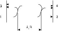
We may make a directional coupler by placing side by side two rectangular metal waveguides having coupling holes in the common wall [1]. Figure 6.7 shows a simple directional coupler having two holes d = lg /4 apart in the broad wall of the waveguides. Let us assume that the coupling factor of a single hole is Bf in the forward direction and Bb in the backward direction.
Passive Transmission Line and Waveguide Devices |
123 |
||||||||||||||||
|
|
|
|
|
|
|
|
|
|
|
|
|
|
|
|
|
|
|
|
|
|
|
|
|
|
|
|
|
|
|
|
|
|
|
|
|
|
|
|
|
|
|
|
|
|
|
|
|
|
|
|
|
|
|
|
|
|
|
|
|
|
|
|
|
|
|
|
|
|
|
|
|
|
|
|
|
|
|
|
|
|
|
|
|
|
|
|
|
|
|
|
|
|
|
|
|
|
|
|
|
|
|
|
|
|
|
|
|
|
|
|
|
|
|
|
|
|
|
|
|
|
|
|
|
|
|
|
|
|
|
|
|
|
|
|
|
|
|
|
|
|
|
|
|
|
|
|
|
|
|
|
|
|
|
|
|
|
|
|
|
|
Figure 6.7 Two-hole waveguide directional coupler.
For example, if a wave is applied to port 1 and its field is equal to 1 in the lower waveguide at a hole, in the upper waveguide the fields of the waves propagating toward ports 3 and 4 are Bb and Bf , respectively. If the coupling factors are small, the fields in the lower waveguide at both holes have nearly equal amplitudes. The two paths from port 1 to port 4 have equal lengths, and the fields strengthen each other at port 4. If the coupling holes are identical, the coupling is in decibels
C = −20 log X2 | Bf | C |
(6.18) |
On the other hand, the paths from port 1 to port 3 have a difference of lg /2 in their lengths. The waves coupled through the holes to port 3 have opposite phases and cancel each other. Hence the directivity D is infinite.
The separation of the holes in the directional coupler of Figure 6.7 is lg /4 only at a single frequency. As the frequency deviates from this frequency, the directivity decreases. The frequency response of the directivity is
D = 20 log |
2 | Bf | |
= 20 log |
| Bf | |
+ 20 log |
1 |
|
| Bb | |1 + e −j 2bd | |
| Bb | |
| cos bd | |
|
(6.19)
The directivity can be interpreted as the sum of the directivity of a single hole and the directivity of the array of holes. A good directivity over a broad band can be achieved by using several coupling holes separated by lg /4 at the center frequency. As before, the coupling and directivity of a multihole coupler can be calculated by summing the fields at ports 3 and 4. By choosing the sizes of the holes properly, different frequency responses, such as the Butterworth or Chebyshev response, can be realized for the directivity [2].
The waveguide junction shown in Figure 6.8 is called the magic T-junction. It operates as a 180° hybrid. A wave applied to port 1 (S) is