

116 Radio Engineering for Wireless Communication and Sensor Applications
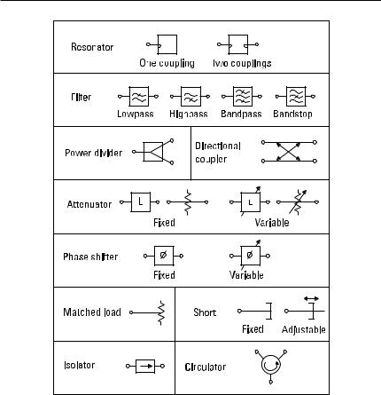
Figure 6.1 Standardized symbols for passive devices.
3.Quasioptical components handle waves propagating in a beam in free space. The dimensions of quasioptical components are larger than a wavelength. They are used in millimeter-wave and submilli- meter-wave systems.
6.1Power Dividers and Directional Couplers
Power dividers and directional couplers are components that split the input signal into two or more output ports. They may also be used as power combiners. Power dividers usually are three-port devices. Directional couplers have four ports and can separate waves propagating into opposite directions on the line. Directional couplers are used in impedance measurement and
Passive Transmission Line and Waveguide Devices |
117 |
for taking a sample of a signal. Hybrids are 3-dB directional couplers with either a 90° or 180° phase difference between their output signals. Hybrids are needed in many mixers, modulators, and demodulators.
6.1.1 Power Dividers
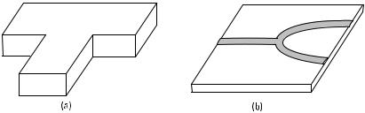
The T-junctions shown in Figure 6.2 are simple power dividers. However, all the ports of a lossless three-port circuit cannot be matched. We can prove this by considering the properties of the scattering matrices. A passive, reciprocal, and matched three-port would have a scattering matrix, as
|
0 |
S12 |
S13 |
4 |
|
[S ] = |
S12 |
0 |
S23 |
(6.1) |
|
|
3S13 |
S23 |
0 |
|
As we stated in Chapter 5, the scattering matrix of a lossless circuit is unitary, from which it follows that
| S12 |2 |
+ | S13 |2 |
= 1 |
(6.2) |
|
| S12 |2 |
+ | S23 |2 |
= 1 |
(6.3) |
|
| S13 |2 |
+ | S23 |2 |
= 1 |
(6.4) |
|
S13* S23 |
= 0 |
(6.5) |
||
S23* S12 |
= 0 |
(6.6) |
||
S12* S13 |
= 0 |
(6.7) |
||
Figure 6.2 T-junctions: (a) a waveguide junction; (b) a microstrip line junction.
118 Radio Engineering for Wireless Communication and Sensor Applications
According to (6.5) through (6.7) at least two of the parameters S12 , S13 , and S23 are zero. However, this is in contradiction with at least one of (6.2) through (6.4). Thus, such a circuit cannot exist.
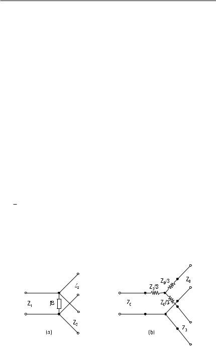
Let us consider the matching problem of a lossless T-junction with an equivalent circuit shown in Figure 6.3(a). The parallel susceptance B represents the reactive fields produced by the discontinuity of the junction. The characteristic impedances of the ports are Z 1 , Z 2 , and Z 3 . Let us assume that B = 0. We then choose Z 2 = Z 3 = 2Z 1 and assume that the ports are terminated with load impedances equal to their characteristic impedances. Now port 1 is matched: The input impedance is Z 1 and the power fed to port 1 is split evenly to the loads of ports 2 and 3. However, ports 2 and 3 are not matched because their input impedance is 2Z 1 /3 (Z 1 and 2Z 1 in parallel) instead of 2Z 1 .
All ports of a three-port divider can be matched by using resistive elements. Figure 6.3(b) shows a matched power divider containing lumped resistors. One half of the power coupled to the input port is absorbed in these resistors.
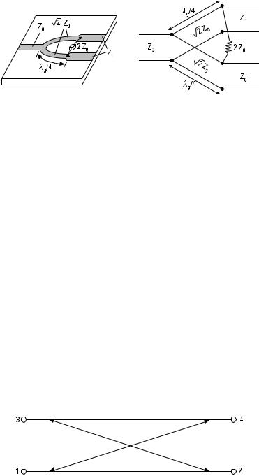
The isolation of the output ports of these power dividers is poor since a part of the power reflected from a mismatched output load is coupled to the other output port. The Wilkinson power divider shown in Figure 6.4 avoids this disadvantage. All the ports are matched to a characteristic impedance Z 0 if the quarter-wave-long sections have a characteristic impedance of √2Z 0 , and the output ports 2 and 3 are connected with a lumped resistor having a resistance 2Z 0 . This circuit is also lossless if the ports are terminated with a matched load, that is, with an impedance of Z 0 .
For all the power dividers discussed so far, the ratio of output powers equals 1. However, this ratio can be chosen freely by modifying the parameters of the circuits.
Figure 6.3 Equivalent circuits of power dividers: (a) lossless T-junction and (b) resistive power divider.
Passive Transmission Line and Waveguide Devices |
119 |
||
|
|
|
|
|
|
|
|
Figure 6.4 Wilkinson power divider.
6.1.2 Coupling and Directivity of a Directional Coupler
Let us consider the directional coupler shown in Figure 6.5 and assume that it is ideal. If a wave is fed from a signal source into port 1, it will couple to ports 2 and 4 but not at all to port 3. Similarly, if port 2 is the input port, ports 1 and 3 are output ports and port 4 is an isolated port. An ideal directional coupler is also lossless, and all of its ports can be matched. If all the ports are terminated with a matched load, the input reflection coefficients are zero. In practice, these properties can be achieved only approximately.
Let us assume that the power coupled into the input port 1 is P 1 and the powers coupled from ports 2, 3, and 4 to the matched terminations are P 2 , P 3 , and P 4 , respectively. The coupling C and directivity D in decibels are defined as
C = 10 log |
P 1 |
|
(6.8) |
P 4 |
|||
D = 10 log |
P 4 |
|
(6.9) |
P 3 |
|||
Usually, most of the input power couples to the termination of the main line at port 2. The coupling describes the power coupled from the main line to the side line and is designed to a value that depends on the
Figure 6.5 Directional coupler.