
- •Radio Engineering for Wireless Communication and Sensor Applications
- •Contents
- •Preface
- •Acknowledgments
- •1 Introduction to Radio Waves and Radio Engineering
- •1.1 Radio Waves as a Part of the Electromagnetic Spectrum
- •1.2 What Is Radio Engineering?
- •1.3 Allocation of Radio Frequencies
- •1.4 History of Radio Engineering from Maxwell to the Present
- •2.2 Fields in Media
- •2.3 Boundary Conditions
- •2.4 Helmholtz Equation and Its Plane Wave Solution
- •2.5 Polarization of a Plane Wave
- •2.6 Reflection and Transmission at a Dielectric Interface
- •2.7 Energy and Power
- •3 Transmission Lines and Waveguides
- •3.1 Basic Equations for Transmission Lines and Waveguides
- •3.2 Transverse Electromagnetic Wave Modes
- •3.3 Transverse Electric and Transverse Magnetic Wave Modes
- •3.4 Rectangular Waveguide
- •3.4.1 TE Wave Modes in Rectangular Waveguide
- •3.4.2 TM Wave Modes in Rectangular Waveguide
- •3.5 Circular Waveguide
- •3.6 Optical Fiber
- •3.7 Coaxial Line
- •3.8 Microstrip Line
- •3.9 Wave and Signal Velocities
- •3.10 Transmission Line Model
- •4 Impedance Matching
- •4.1 Reflection from a Mismatched Load
- •4.2 Smith Chart
- •4.3 Matching Methods
- •4.3.1 Matching with Lumped Reactive Elements
- •4.3.4 Resistive Matching
- •5 Microwave Circuit Theory
- •5.1 Impedance and Admittance Matrices
- •5.2 Scattering Matrices
- •5.3 Signal Flow Graph, Transfer Function, and Gain
- •6.1 Power Dividers and Directional Couplers
- •6.1.1 Power Dividers
- •6.1.2 Coupling and Directivity of a Directional Coupler
- •6.1.3 Scattering Matrix of a Directional Coupler
- •6.1.4 Waveguide Directional Couplers
- •6.1.5 Microstrip Directional Couplers
- •6.2 Ferrite Devices
- •6.2.1 Properties of Ferrite Materials
- •6.2.2 Faraday Rotation
- •6.2.3 Isolators
- •6.2.4 Circulators
- •6.3 Other Passive Components and Devices
- •6.3.1 Terminations
- •6.3.2 Attenuators
- •6.3.3 Phase Shifters
- •6.3.4 Connectors and Adapters
- •7 Resonators and Filters
- •7.1 Resonators
- •7.1.1 Resonance Phenomenon
- •7.1.2 Quality Factor
- •7.1.3 Coupled Resonator
- •7.1.4 Transmission Line Section as a Resonator
- •7.1.5 Cavity Resonators
- •7.1.6 Dielectric Resonators
- •7.2 Filters
- •7.2.1 Insertion Loss Method
- •7.2.2 Design of Microwave Filters
- •7.2.3 Practical Microwave Filters
- •8 Circuits Based on Semiconductor Devices
- •8.1 From Electron Tubes to Semiconductor Devices
- •8.2 Important Semiconductor Devices
- •8.2.1 Diodes
- •8.2.2 Transistors
- •8.3 Oscillators
- •8.4 Amplifiers
- •8.4.2 Effect of Nonlinearities and Design of Power Amplifiers
- •8.4.3 Reflection Amplifiers
- •8.5.1 Mixers
- •8.5.2 Frequency Multipliers
- •8.6 Detectors
- •8.7 Monolithic Microwave Circuits
- •9 Antennas
- •9.1 Fundamental Concepts of Antennas
- •9.2 Calculation of Radiation from Antennas
- •9.3 Radiating Current Element
- •9.4 Dipole and Monopole Antennas
- •9.5 Other Wire Antennas
- •9.6 Radiation from Apertures
- •9.7 Horn Antennas
- •9.8 Reflector Antennas
- •9.9 Other Antennas
- •9.10 Antenna Arrays
- •9.11 Matching of Antennas
- •9.12 Link Between Two Antennas
- •10 Propagation of Radio Waves
- •10.1 Environment and Propagation Mechanisms
- •10.2 Tropospheric Attenuation
- •10.4 LOS Path
- •10.5 Reflection from Ground
- •10.6 Multipath Propagation in Cellular Mobile Radio Systems
- •10.7 Propagation Aided by Scattering: Scatter Link
- •10.8 Propagation via Ionosphere
- •11 Radio System
- •11.1 Transmitters and Receivers
- •11.2 Noise
- •11.2.1 Receiver Noise
- •11.2.2 Antenna Noise Temperature
- •11.3 Modulation and Demodulation of Signals
- •11.3.1 Analog Modulation
- •11.3.2 Digital Modulation
- •11.4 Radio Link Budget
- •12 Applications
- •12.1 Broadcasting
- •12.1.1 Broadcasting in Finland
- •12.1.2 Broadcasting Satellites
- •12.2 Radio Link Systems
- •12.2.1 Terrestrial Radio Links
- •12.2.2 Satellite Radio Links
- •12.3 Wireless Local Area Networks
- •12.4 Mobile Communication
- •12.5 Radionavigation
- •12.5.1 Hyperbolic Radionavigation Systems
- •12.5.2 Satellite Navigation Systems
- •12.5.3 Navigation Systems in Aviation
- •12.6 Radar
- •12.6.1 Pulse Radar
- •12.6.2 Doppler Radar
- •12.6.4 Surveillance and Tracking Radars
- •12.7 Remote Sensing
- •12.7.1 Radiometry
- •12.7.2 Total Power Radiometer and Dicke Radiometer
- •12.8 Radio Astronomy
- •12.8.1 Radio Telescopes and Receivers
- •12.8.2 Antenna Temperature of Radio Sources
- •12.8.3 Radio Sources in the Sky
- •12.9 Sensors for Industrial Applications
- •12.9.1 Transmission Sensors
- •12.9.2 Resonators
- •12.9.3 Reflection Sensors
- •12.9.4 Radar Sensors
- •12.9.5 Radiometer Sensors
- •12.9.6 Imaging Sensors
- •12.10 Power Applications
- •12.11 Medical Applications
- •12.11.1 Thermography
- •12.11.2 Diathermy
- •12.11.3 Hyperthermia
- •12.12 Electronic Warfare
- •List of Acronyms
- •About the Authors
- •Index

50 Radio Engineering for Wireless Communication and Sensor Applications
Table 3.2
Standard Waveguides
Abbreviation |
a [mm] |
b [mm] |
f c [GHz] |
Range [GHz] |
|
|
|
|
|
WR-90 |
22.86 |
10.16 |
6.56 |
8.2–12.4 |
WR-75 |
19.05 |
9.53 |
7.87 |
10–15 |
WR-62 |
15.80 |
7.90 |
9.49 |
12.4–18 |
WR-51 |
12.95 |
6.48 |
11.6 |
15–22 |
WR-42 |
10.67 |
4.32 |
14.1 |
18–26.5 |
WR-34 |
8.64 |
4.32 |
17.4 |
22–33 |
WR-28 |
7.11 |
3.56 |
21.1 |
26.5–40 |
WR-22 |
5.69 |
2.84 |
26.3 |
33–50 |
WR-19 |
4.78 |
2.39 |
31.4 |
40–60 |
WR-15 |
3.76 |
1.88 |
39.9 |
50–75 |
WR-12 |
3.10 |
1.55 |
48.4 |
60–90 |
WR-10 |
2.54 |
1.27 |
59.0 |
75–110 |
WR-8 |
2.03 |
1.02 |
73.8 |
90–140 |
|
|
|
|
|
0.1 dB/cm, the power absorbed into the walls of the waveguide is about 240 W/cm at the maximum power. If the load reflects some of the power, the maximum field strength is due to the standing wave higher than in the matched case. Then, the maximum power is lower than that calculated above.
3.4.2 TM Wave Modes in Rectangular Waveguide
TM wave modes have no longitudinal magnetic field component, Hz = 0. The solution of the longitudinal electric field has a form of
Ez = B sin (k 1 x ) sin (k 2 y )
The other field components are
Hx = |
vek |
2 |
|
|
|||
j |
|
|
|
|
|
B sin (k 1 x ) cos (k 2 y ) |
|
|
k 2c |
|
|
|
|||
|
|
|
|
|
|
|
|
|
|
ve k 1 |
|
||||
Hy = −j |
|
|
|
|
B cos (k 1 x ) sin (k 2 y ) |
||
k 2c |
|
|
|
||||
|
|
|
|
|
|
|
Ex = Z TM Hy
(3.57)
(3.58)
(3.59)
(3.60)

|
|
|
|
Transmission Lines and Waveguides |
51 |
||||||||||||||||
|
|
|
|
|
|
|
|
|
|
|
|
|
|
|
|
|
|
|
|
|
|
|
|
|
|
|
|
|
|
|
|
|
|
|
|
|
|
|
|
|
|
|
|
|
|
|
|
|
|
|
|
|
|
|
|
|
|
|
|
|
|
|
|
|
|
|
|
|
|
|
|
|
|
|
|
|
|
|
|
|
|
|
|
|
|
|
|
|
|
|
|
|
|
|
|
|
|
|
|
|
|
|
|
|
|
|
|
|
|
|
|
|
|
|
|
|
|
|
|
|
|
|
|
|
|
|
|
|
|
|
|
|
|
|
|
|
|
|
|
|
|
|
|
|
|
|
|
|
|
|
|
|
|
|
|
|
|
|
|
|
|
|
|
|
|
|
|
|
|
|
|
|
|
|
|
|
|
|
|
|
|
|
|
|
|
|
|
|
|
|
|
|
|
|
|
|
|
|
|
|
|
|
|
|
|
|
|
|
|
|
|
|
|
|
|
|
|
|
|
|
|
|
|
|
|
|
|
|
|
|
|
|
|
|
|
|
|
|
|
|
|
|
|
|
|
|
|
|
|
|
|
|
|
|
|
|
|
|
|
|
|
|
|
|
|
|
|
|
|
|
|
|
|
|
|
|
|
|
|
|
|
|
|
|
|
|
|
|
|
|
|
|
|
|
|
|
|
|
|
|
|
|
|
|
|
|
|
|
|
|
|
|
|
|
|
|
|
|
|
|
|
|
|
|
|
|
|
|
|
|
|
|
|
|
|
|
|
|
|
|
|
|
|
|
|
|
|
|
|
|
|
|
|
|
|
|
|
|
|
|
|
|
|
|
|
|
|
|
|
|
|
|
|
|
|
|
|
|
|
|
|
|
|
|
|
|
|
|
|
|
|
|
|
|
|
|
|
|
|
|
|
|
|
|
|
|
|
|
|
|
|
|
|
|
|
|
|
|
|
|
|
|
|
|
|
|
|
|
|
|
|
|
|
|
|
|
|
|
|
|
|
|
|
|
|
|
|
|
|
|
|
|
|
|
|
|
|
|
|
|
|
|
|
|
|
|
|
|
|
|
|
|
|
|
|
|
|
|
|
|
|
|
|
|
|
|
|
|
|
|
|
|
|
|
|
|
|
|
|
|
|
|
|
|
|
|
|
|
|
|
|
|
|
|
|
|
|
|
|
|
|
|
|
|
|
|
|
|
|
|
|
|
|
|
|
|
|
|
|
|
|
|
|
|
|
|
|
|
|
|
|
|
|
|
|
|
|
|
|
|
|
|
|
|
|
|
|
|
|
|
|
|
|
|
|
|
|
|
|
|
|
|
|
|
|
|
|
|
|
|
|
|
|
|
|
|
|
|
|
|
|
|
|
|
|
|
|
|
|
|
|
|
|
|
|
|
|
|
|
|
|
|
|
|
|
|
|
|
|
|
|
|
|
|
|
|
|
|
|
|
|
|
|
|
|
|
|
|
|
|
|
|
|
|
|
|
|
|
|
|
|
|
|
|
|
|
|
|
|
|
|
|
|
|
|
|
|
|
|
|
|
|
|
|
|
|
|
|
|
|
|
|
|
|
|
|
|
|
|
|
|
|
|
|
|
|
|
|
|
|
|
|
|
|
|
|
|
|
|
|
|
|
|
|
|
|
|
|
|
|
|
|
|
|
|
|
|
|
|
|
|
|
|
|
|
|
|
|
|
|
|
|
|
|
|
|
|
|
|
|
|
|
|
|
|
|
|
|
|
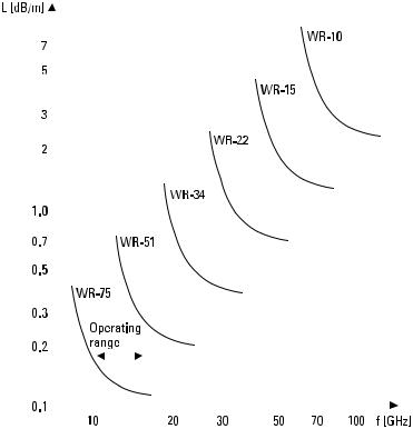
Figure 3.6 Attenuation of standard waveguides.
Ey = −Z TM Hx |
(3.61) |
The wave impedance of TM modes is
Z TM = h√ |
1 − ( f c /f )2 |
(3.62) |
From boundary conditions it follows that the equations for the cutoff wavelength and cutoff frequency are the same as those for the TE wave modes. Now, both indices n and m have to be nonzero. The TM wave mode having the lowest cutoff frequency is TM11 . Although TM11 and TE11 wave modes have equal cutoff frequencies, their field distributions are different. Figure 3.7 shows transverse field distributions of some TE and TM wave modes.