


40 Radio Engineering for Wireless Communication and Sensor Applications
modes. Every mode has its own propagation characteristics: velocity, attenuation, and cutoff frequency. Because different modes propagate at different velocities, signals may be distorted due to the multimode propagation. Using the waveguide at low enough frequencies, so that only one mode—the dominant or fundamental mode—can propagate along the waveguide, prevents this multimode distortion.
3.2 Transverse Electromagnetic Wave Modes
In lossless and, with a good approximation, in low-loss two-conductor transmission lines, as in coaxial lines, fields can propagate as transverse electromagnetic (TEM) waves. TEM waves have no longitudinal field components. TEM waves may propagate at all frequencies, so the TEM mode has no cutoff frequency.
When Ez = 0 and Hz = 0, it follows from (3.5) through (3.8) that the x - and y -components of the fields are also zero, unless
g 2 + v 2me = 0 |
(3.13) |
Therefore, the propagation constant of a TEM wave is
g = ± jv √ |
|
= ± j |
2p |
= ± jb |
(3.14) |
|
me |
||||||
l |
||||||
|
|
|
|
|
The velocity v p is independent of frequency, assuming that the material parameters e and m are independent of frequency:
v p = |
v |
= |
1 |
(3.15) |
||
|
|
|
||||
b |
√me |
|||||
|
|
|
||||
Thus, there is no dispersion, and the TEM wave in a transmission line propagates at the same velocity as a wave in free space having the same e and m as the insulator of the transmission line. The wave equations for a TEM wave are
=2 |
E = 0 |
(3.16) |
xy |
|
|
=2 |
H = 0 |
(3.17) |
xy |
|
|

Transmission Lines and Waveguides |
41 |
The fields of a wave propagating along the z direction satisfy the equation
E x |
= − |
E y |
= h |
(3.18) |
|
Hy |
Hx |
||||
|
|
|
where h = √m /e is the wave impedance.
Laplace’s equations, (3.16) and (3.17), are valid also for static fields. In electrostatics, the electric field may be presented as the gradient of the scalar transverse potential:
E (x , y ) = −=xy F(x , y ) |
(3.19) |
Because = × =f = 0, the transverse curl of the electric field must vanish in order for (3.19) to be valid. Here this is the case, because
=xy × E = −jvm Hz uz = 0 |
(3.20) |
where uz is a unit vector pointing in the direction of the positive z -axis. Gauss’ law in a sourceless space states that = ? D = e=xy ? E = 0. From this and (3.19) it follows that F(x , y ) is also a solution of Laplace’s equation, or
=2 |
F(x , y ) = 0 |
(3.21) |
xy |
|
|
The voltage of a two-conductor line is
|
2 |
|
|
|
V 12 = |
E |
E ? d l = F1 |
− F2 |
(3.22) |
|
||||
|
1 |
|
|
|
where F1 and F2 are the potentials of the conductors. From Ampe`re’s law, the current of the line is
I = RH ? d l |
(3.23) |
G |
|
where G is a closed line surrounding the conductor.
42 Radio Engineering for Wireless Communication and Sensor Applications
3.3Transverse Electric and Transverse Magnetic Wave Modes
A wave mode may have also longitudinal field components in addition to the transverse components. Transverse electric (TE) modes have Ez = 0 but a nonzero longitudinal magnetic field Hz . Transverse magnetic (TM) modes have Hz = 0 and a nonzero Ez .
From (3.4) it follows for a TE mode
=2 |
H |
z |
= −( g2 |
+ v 2me ) H |
z |
= −k |
2 |
H |
z |
(3.24) |
xy |
|
|
|
|
c |
|
|
Correspondingly, for a TM mode
=2 |
E |
z |
= −( g2 + v2me ) E |
z |
= −k |
2 |
E |
z |
(3.25) |
xy |
|
|
|
c |
|
|
The coefficient k c is solved from (3.24) or (3.25) using the boundary conditions set by the waveguide. For a given waveguide, an infinite number of k c values can usually be found. Each k c corresponds to a propagating wave mode. We can prove that in the case of a waveguide such as a rectangular or circular waveguide, in which a conductor surrounds an insulator, k c is always a positive real number.
The propagation constant is
g = √ |
|
|
k 2c − v 2me |
(3.26) |
If the insulating material is lossless, v 2me is real. The frequency at which v 2me = k2c is called the cutoff frequency:
f c = |
|
k c |
(3.27) |
||||
|
|
|
|
|
|||
2p√me |
|||||||
|
|
||||||
The corresponding cutoff wavelength is |
|
||||||
l c = |
2p |
|
(3.28) |
||||
k c |
|||||||
|
|
|
|||||
At frequencies below the cutoff frequency, f < f c , no wave can propagate. The field attenuates rapidly and has an attenuation constant
Transmission Lines and Waveguides |
43 |
|||||||
|
|
|
|
|
|
|
|
|
|
2p |
|
|
f |
2 |
|
||
g = a = |
√1 − S |
D |
(3.29) |
|||||
l c |
f c |
|||||||
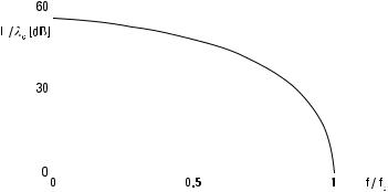
At frequencies much below the cutoff frequency, f << f c , the attenuation constant is a = 2p /lc or 2p nepers (54.6 dB) per cutoff wavelength. Figure 3.2 shows the attenuation at frequencies below the cutoff frequency.
At frequencies higher than the cutoff frequency, f > f c , waves can propagate and the propagation constant g is complex. In a lossless line, g is imaginary:
|
l |
√ |
|
|
|
|
|
|
|
S f |
D |
|
|||
|
2p |
|
|
|
f c |
2 |
|
g = jbg = j |
|
|
1 − |
|
|
|
(3.30) |
where l is the wavelength in free space composed of the same material as the insulator of the line. The wavelength in the line is
l g = |
2p |
= |
|
|
l |
|
|
(3.31) |
|
|
|
|
|
||||
|
√1 |
|
|
|
||||
|
bg |
− ( f c /f ) |
2 |
|||||
|
|
|
|
|
|
|||
Figure 3.3 shows how the wavelength l g depends on frequency. The phase velocity (see Section 3.9) is
|
v p = |
|
|
v |
|||||
|
|
|
|
|
(3.32) |
||||
|
|
|
|||||||
|
|
|
|
||||||
|
|
√1 − ( f c /f )2 |
|||||||
|
|
|
|
|
|
|
|
|
|
|
|
|
|
|
|
|
|
|
|
|
|
|
|
|
|
|
|
|
|
|
|
|
|
|
|
|
|
|
|
|
|
|
|
|
|
|
|
|
|
|
|
|
|
|
|
|
|
|
|
|
|
|
|
|
|
|
|
|
|
|
|
|
|
|
|
|
|
|
|
Figure 3.2 Attenuation of TE and TM waves below the cutoff frequency in a lossless waveguide.