Jordan M.Computational aspects of motor control and motor learning

optimization of the following sum-of-squared-error cost function:

where u^[n , 1] denotes the controller output.

Example

Consider the rst-order plant:

As we have seen previously, the inverse model for this plant is linear in the estimated state and the desired output (cf. Equation 15). Let us assume that we do not know the appropriate values for the coe cients in the inverse model, thus we replace them with unknown values v1 and v2:

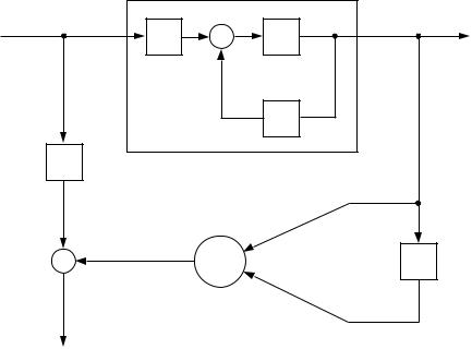
This equation is linear in the unknown parameters, thus we can use the LMS algorithm to learn the values of v1 and v2. We rst shift the time index in Equation 42 to write the inverse model in terms of the current plant output (y[n]). This requires delaying the control input and the state estimate by one time step. Connecting the LMS unit to the plant with the appropriate delays in place yields the wiring diagram in Figure 19. Note that we assume that the state is estimated by feedback from the plant, thus, the delayed state x[n , 1] is estimated by the delayed plant output y[n , 1] (cf. Equation 16). The inputs to the LMS processing unit are the plant output y[n] and the delayed plant output y[n , 1]. The target for the LMS unit is the delayed plant input u[n , 1]. Note that if the unit is equipped with a bias, the bias value will converge to zero because it is not needed to represent the inverse model for this plant.

The nonconvexity problem

The direct inverse modeling approach is well-behaved for linear systems and indeed can be shown to converge to correct parameter estimates for such systems under certain conditions (Goodwin & Sin, 1984). For nonlinear systems, however, a di culty arises that is related to the general \degrees-of-freedom problem" in motor control (Bernstein, 1967). The problem is due to a particular form of redundancy in nonlinear systems (Jordan, 1992). In such systems, the \optimal" parameter estimates (i.e., those that minimize the cost function in Equation 40) in fact yield an incorrect controller.

41

Figure 19: An example of the direct inverse modeling approach. An LMS processing unit is connected to the rst order plant. The bias has been omitted for simplicity.

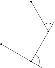
To illustrate, let us consider the planar kinematic arm shown in Figure 20. The arm has three joint angles, which we denote by 1, 2, and 3. The tip of the arm can be described by a pair of Cartesian coordinates, which we denote by y1 and y2. For every vector of joint angles there is a corresponding Cartesian position vector y. The mapping from to y is a nonlinear function known as the forward kinematics of the arm.

Suppose that we use the direct inverse modeling approach to learn the inverse kinematics of the arm; that is, the mapping from y to (cf. Kuperstein, 1988). Data for the learning algorithm are obtained by trying random joint angle con gurations and observing the corresponding position of the tip of the arm. A nonlinear supervised learning algorithm is used to learn the mapping from tip positions to joint angles. Figure 21 shows the results of a simulation of this approach for the planar arm. The gure is an error vectoreld, that is, the tail of each arrow is a desired position, and the head of each arrow is the position produced by utilizing the inverse model to produce a set

42

(y1 , y2 )

θ3

θ1

Figure 20: A three-joint planar arm.

of joint angles. As can be observed, there are substantial errors throughout the workspace.

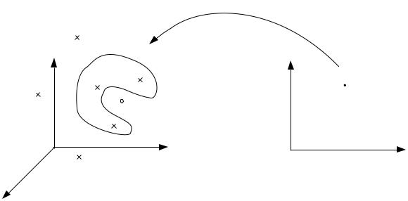
It is possible to rule out a number of possible explanations for the errors. The errors are not explained by possible local minima, by insu cient training time, or by poor approximation capability of the inverse model (Jordan & Rumelhart, 1992). The particular inverse model used in the simulation was a feedforward neural network trained with backpropagation, but it can be shown that any least-squares-based nonlinear approximator would give a similar result. To understand the di culty, let us consider the direct inverse modeling approach geometrically, as shown in Figure 22. The gure shows the joint space on the left and the Cartesian space on the right. The arm is a redundant kinematic system; that is, to every tip position inside the workspace, there are an in nite set of joint angle con gurations that achieve that position. Thus, to every point on the right side of the gure, there is a corresponding region (the inverse image) on the left. The direct inverse modeling approach samples randomly in joint space, observes the corresponding points in Cartesian space, and learns the mapping in the reverse direction. Let us suppose that three sample points happen to fall in a particular inverse image (see Figure 22). All three of these points correspond to a single point in Cartesian space, thus, the direct inverse learner is presented with data that are one-to- many: A single input maps to three di erent target outputs. The optimal least-squares solution is to produce an output that is an average of the three

43

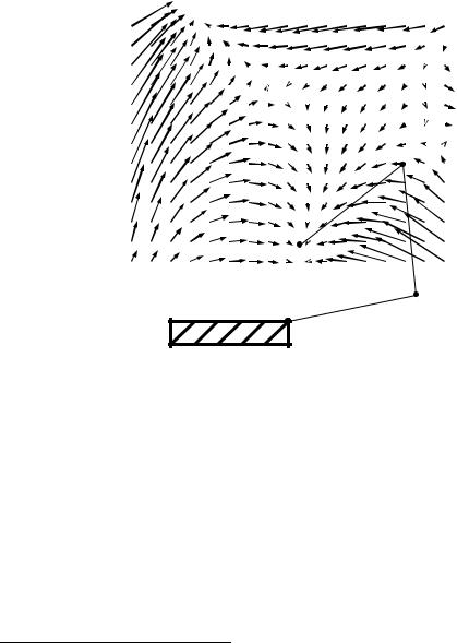
Figure 21: Near-asymptotic performance of direct inverse modeling. Each vector represents the error at a particular position in the workspace.

targets. If the inverse image has a nonconvex shape, as shown in the gure, then the average of the three targets lies outside of the inverse image and is therefore not a solution.

It is easy to demonstrate that linear systems always have convex inverse images, thus the nonconvexity problem does not arise for such systems.10 The problem does arise for nonlinear systems, however. In particular, Figure 23 demonstrates that the problem arises for the planar kinematic arm. The gure shows two particular joint angle con gurations that lie in the same inverse image (i.e., map into the same Cartesian position). The gure also shows the

10 Let y = f (x) be a linear function, and consider a particular point y in the range of f. The convex combination of any two points x1 and x2 that lie in the inverse image of y also lies in the inverse image of y :

f ( x1 + (1 , )x2) = f (x1) + (1 , )f(x2)

=y + (1 , )y

=y ;

where 0 < < 1. Thus the inverse image is a convex set.

44

Figure 22: The convexity problem. The region on the left is the inverse image of the point on the right. The arrow represents the direction in which the mapping is learned by direct inverse modeling. The three points lying inside the inverse image are averaged by the learning procedure, yielding the vector represented by the small circle. This point is not in the inverse image, because the inverse image is not convex, and is therefore not a solution.

joint-space average of these two con gurations (the dashed con guration in thegure). An average of two points lies on the straight line joining the points, thus the fact that the average con guration does not itself lie in the inverse image (i.e., does not map into the same Cartesian position) demonstrates that the inverse image is nonconvex. Interestingly, the Cartesian error observed in Figure 23 is essentially the same error as that observed in the corresponding position of the error vector eld in Figure 21. This provides support for the assertion that the error vector eld is due to the nonconvexities of the inverse kinematics.

Feedback error learning

Kawato, Furukawa and Suzuki (1987) have developed a direct approach to motor learning that avoids some of the di culties associated with direct inverse modeling. Their approach, known as feedback error learning, makes use

45

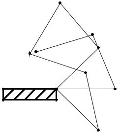
Figure 23: The nonconvexity of inverse kinematics. The dotted con guration is an average in joint space of the two solid con gurations.

of a feedback controller to guide the learning of the feedforward controller. Consider the composite feedback-feedforward control system discussed earlier (cf. Figure 9), in which the total control signal is the sum of the feedforward component and the feedback component:

u[n] = uf f [n] + uf b [n]:

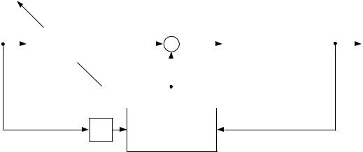
In the context of a direct approach to motor learning, the signal u[n] is the target for learning the feedforward controller (cf. Figure 18). The error between the target and the feedforward control signal is (u[n],uf f [n]), which in the current case is simply uf b[n]. Thus an error for learning the feedforward controller can be provided by the feedback control signal (see Figure 24).

An important di erence between feedback error learning and direct inverse modeling regards the signal used as the controller input. In direct inverse modeling the controller is trained \o -line;" that is, the input to the controller for the purposes of training is the actual plant output, not the desired plant output. For the controller to actually participate in the control process, it must receive the desired plant output as its input. The direct inverse modeling approach therefore requires a switching process|the desired plant output must be switched in for the purposes of control and the actual plant output must be switched in for the purposes of training. The feedback error learning approach provides a more elegant solution to this problem. In feedback error learning,

46

Feedback

D

Controller

Figure 24: The feedback error learning approach to learning a feedforward controller. The feedback control signal is the error term for learning the feedforward controller.

the desired plant output is used for both control and training. The feedforward controller is trained \on-line;" that is, it is used as a controller while it is being trained. Although the training data that it receives|pairs of actual plant inputs and desired plant outputs|are not samples of the inverse dynamics of the plant, the system nonetheless converges to an inverse model of the plant because of the error-correcting properties of the feedback controller.

By utilizing a feedback controller, the feedback error learning approach also solves another problem associated with direct inverse modeling. Direct inverse modeling is not goal directed; that is, it is not sensitive to particular output goals (Jordan & Rosenbaum, 1989). This is seen by simply observing that the goal signal (y [n + 1]) does not appear in Figure 18. The learning process samples randomly in the control space, which may or may not yield a plant output near any particular goal. Even if a particular goal is speci ed before the learning begins, the direct inverse modeling procedure must search throughout the control space until an acceptable solution is found. In the feedback error learning approach, however, the feedback controller serves to guide the system to the correct region of the control space. By using a feedback controller, the system makes essential use of the error between the desired plant output and the actual plant output to guide the learning. This fact links the feedback error learning approach to the indirect approach to motor learning that we discuss in the following section. In the indirect approach, the learning algorithm is based directly on the output error.

47

Distal supervised learning

In this section we describe an indirect approach to motor learning known as distal supervised learning. Distal supervised learning avoids the nonconvexity problem and also avoids certain other problems associated with direct approaches to motor learning (Jordan, 1990; Jordan & Rumelhart, 1992). In distal supervised learning, the controller is learned indirectly, through the intermediary of a forward model of the plant. The forward model must itself be learned from observations of the inputs and outputs of the plant. The distal supervised learning approach is therefore composed of two interacting processes, one process in which the forward model is learned and another process in which the forward model is used in the learning of the controller.

In the case of a linear plant, the distal supervised learning approach is a cross between two techniques from adaptive control theory: indirect self-tuning control and indirect model reference adaptive control (Astrom & Wittenmark, 1989). Let us begin by describing the basic idea of indirect self-tuning control, to provide some insight into how a forward model can be used as an intermediary in the learning of an inverse model. Consider once again the rst-order example (Equation 41). Suppose that instead of learning an inverse model of the plant directly, the system rst learns a forward model of the plant. We assume a parameterized forward plant model of the following form:

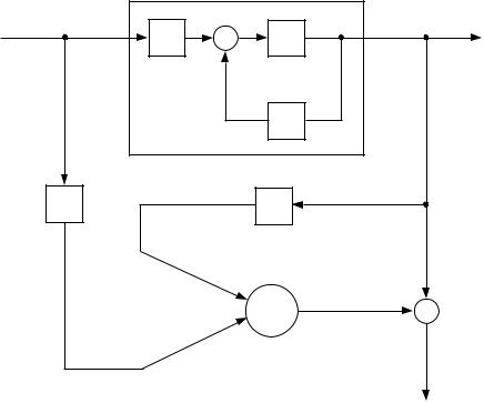
where the weights w1 and w2 are unknown parameters. This equation is linear in the unknown parameters, thus the LMS algorithm is applicable. As in the previous section, we shift the time index backward by one time step to express the model in terms of the current plant output y[n]. This yields the wiring diagram shown in Figure 25. The forward model is an LMS processing unit with inputs u[n , 1] and y[n , 1], where y[n , 1] is the estimate x^[n , 1]. The output of the LMS unit is the predicted plant output y^[n] and the target for the learning algorithm is the actual plant output y[n]. By minimizing the prediction error (y[n] , y^[n]), the system adjusts the weights in the forward model.

Let us suppose that the learner has acquired a perfect forward model; that is, the predicted plant output is equal to the actual plant output for all states and all inputs. Equation 43 can now be inverted algebraically to provide an inverse model of the following form:

48

Figure 25: An example of the learning of the forward model in the distal supervised learning approach. An LMS processing unit is connected to therst order plant. The bias has been omitted for simplicity.

Note that in this equation, the weights of the forward model are being used to construct the inverse model. If the forward model is perfect, that is, if w1 is equal to .5 and w2 is equal to .4, then the inverse model is also perfect|the coe cients in Equation 44 are 1.25 and 2.5 (cf. Equation 15).

The nonlinear case

In the case of a linear plant, the di erences between the direct approach to learning an inverse model and the indirect approach to learning an inverse model are relatively minor. Essentially, the choice is between performing the algebra rst and then the learning, or the learning rst and then the algebra. In the nonlinear case, however, the di erences are much more salient. Indeed, it is not entirely clear how to proceed in the nonlinear case, given that nonlin-

49

ear plant models are generally nonlinear in the parameters and are therefore di cult to invert algebraically.

To see how to proceed, let us reconsider the notion of an inverse model of the plant. Rather than de ning an inverse model as a particular transformation from plant outputs to plant inputs, let us de ne an inverse model as any transformation that when placed in series with the plant yields the identity transformation. That is, an inverse model is any system that takes an input y [n + 1] (at time n) and provides a control signal to the plant such that the plant output (at time n +1) is equal to y [n +1]. This implicit de nition of an inverse model recognizes that there may be more than one inverse model of the plant. Moreover, this de nition suggests an alternative approach to training an inverse model. Suppose that we consider the controller and the plant together as a single composite system that transforms a desired plant output into an actual plant output. An indirect approach to training the controller is to train this composite system to be the identity transformation.

Stated in this manner, this indirect approach seems unrealizable, because learning algorithms require access to the internal structure of the system that they are training, and internal structure is precisely what is lacking in the case of the unknown physical plant. There is a way out, however, which involves using an internal forward model of the plant rather than the plant itself. This is the essence of the distal supervised learning approach, as illustrated diagrammatically in Figure 26. There are two interwoven processes depicted in the gure. One process involves the acquisition of an internal forward model of the plant. The forward model is a mapping from states and inputs to predicted plant outputs and it is trained using the prediction error (y[n] , y^[n]). The second process involves training the controller. This is accomplished in the following manner. The controller and the forward model are joined together and are treated as a single composite learning system. Using a nonlinear supervised learning algorithm, the composite system is trained to be an identity transformation. That is, the entire composite learning system (the system inside the dashed box in the gure) corresponds to the box labelled \Learner" in Figure 17. During this training process, the parameters in the forward model are held xed. Thus the composite learning system is trained to be an identity transformation by a constrained learning process in which some of the parameters inside the system are held xed. By allowing only the controller parameters to be altered, this process trains the controller indirectly.11

11 It has been suggested (Miall, Weir, Wolpert, & Stein, in press) that the distal supervised learning approach requires using the backpropagation algorithm of Rumelhart, Hinton, and Williams (1986). This is not the case; indeed, a wide variety of supervised learning algorithms are applicable. The only requirement of the algorithm is that it obey an \architectural

50