

Jordan M.Computational aspects of motor control and motor learning
.pdfinverse model of the plant.8 Thus an error-correcting feedback control system with high gain is equivalent to an open-loop feedforward system that utilizes an explicit inverse model. This is true even though the feedback control system is clearly not computing an explicit plant inverse. We can think of the feedback loop as implicitly inverting the plant.
In many real feedback systems, it is impractical to allow the gain to grow large. One important factor that limits the magnitude of the gain is the presence of delays in the feedback loop, as we will see in the following section. Other factors have to do with robustness to noise and disturbances. It is also the case that some plants|so-called \nonminimum phase" plants| are unstable if the feedback gain is too large (Astrom & Wittenmark, 1984). Nonetheless, it is still useful to treat a feedback control system with a nite gain K as computing an approximation to a inverse model of the plant. This approximation is ideally as close as possible to a true inverse of the plant, subject to constraints related to stability and robustness.
The notion that a high-gain feedback control system computes an approximate inverse of the plant makes intuitive sense as well. Intuitively, a high-gain controller corrects errors as rapidly as possible. Indeed, as we saw in Figure 6, as the gain of the feedback controller grows, its performance approaches that of a deadbeat controller (Figure 3(b)).
It is also worth noting that the system shown in Figure 8 can be considered in its own right as an implementation of a feedforward control system. Suppose that the replica of the plant in the feedback loop in Figure 8 is implemented literally as an internal forward model of the plant. If the forward model is an accurate model of the plant, then in the limit of high gain this internal loop is equivalent to an explicit inverse model of the plant. Thus the internal loop is an alternative implementation of a feedforward controller. The controller is an open-loop feedforward controller because there is no feedback from the actual plant to the controller. Note that this alternative implementation of an open-loop feedforward controller is consistent with our earlier characterization of feedforward control: (1) The control system shown in Figure 8 requires explicit knowledge of the plant dynamics (the internal forward model); (2) the performance of the controller is sensitive to inaccuracies in the plant model (the loop inverts the forward model, not the plant); and (3) the controller does not correct for unanticipated disturbances (there is no feedback from the
8 In fact, the mathematical argument just presented is not entirely correct. The limiting process in our argument is well-de ned only if the discrete-time dynamical system is obtained by approximating an underlying continuous-time system and the time step of the approximation is taken to zero as the gain is taken to in nity. Readers familiar with the Laplace transform will be able to justify the argument in the continuous-time domain.
21
y* |
|
Feedforward |
uff [n] + |
|
u |
|
|
|
y |
[n] |
||
[n +1] |
|
|
[n ] |
|
|
Plant |
|
|||||
|
|
Controller |
|
|
|
|
|
|
|
|
|
|
|
|
+ |
|
|
|
|
||||||
|
|
|
|
|
|
|
|
|
||||
|
|
|
ufb[n] |
|
|
|
|
|
||||
|
|
|
|
|
|
|
|
|
|
|
||
|
|
|
|
|
|
|
|
|
|
|
||
|
|
|
|
|
|
|
|
|
|
|
|
|
Feedback
D
Controller
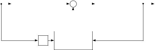
Figure 9: A composite control system composed of a feedback controller and a feedforward controller.
actual plant output).
Composite control systems
Because feedforward control and error-correcting feedback control have complementary strengths and weaknesses, it is sensible to consider composite control systems that combine these two kinds of control. There are many ways that feedforward and feedback can be combined, but the simplest scheme| that of adding the two control signals|is generally a reasonable approach. Justi cation for adding the control signals comes from noting that because both kinds of control can be thought of as techniques for computing a plant inverse, the sum of the control signals is a sensible quantity.
Figure 9 shows a control system that is composed of a feedforward controller and an error-correcting feedback controller in parallel. The control signal in this composite system is simply the sum of the feedforward control signal and the feedback control signal:
u[n] = uf f [n] + uf b [n]:
If the feedforward controller is an accurate inverse model of the plant, and if there are no disturbances, then there is no error between the plant output and the desired output. In this case the feedback controller is automatically silent. Errors at the plant output, whether due to unanticipated disturbances or due to inaccuracies in the feedforward controller, are corrected by the feedback controller.
22
Delay
The delays in the motor control system are signi cant. Estimates of the delay in the visuomotor feedback loop have ranged from 100 to 200 milliseconds (Keele & Posner, 1968; Carlton, 1981). Such a large value of delay is clearly signi cant in reaching movements, which generally last from 250 milliseconds to a second or two.
Many arti cial control systems are implemented with electrical circuits and fast-acting sensors, such that the delays in the transmission of signals within the system are insigni cant when compared to the time constants of the dynamical elements of the plant. In such cases the delays are often ignored in the design and analysis of the controller. There are cases, however, including the control of processes in a chemical plant and the control of the ight of a spaceship, in which the delays are signi cant. In this section we make use of some of the ideas developed in the study of such problems to describe the e ects of delays and to present tools for dealing with them.
What is the e ect of delay on a control system? The essential e ect of delay is that it generally requires a system to be operated with a small gain in the feedback loop. In a system with delay, the sensory reading that is obtained by the controller re ects the state of the system at some previous time. The control signal corresponding to that sensory reading may no longer be appropriate for the current state of the plant. If the closed-loop system is oscillatory, for example, then the delayed control signal can be out of phase with the true error signal and may contribute to the error rather than correct it. Such an out-of-phase control signal can destabilize the plant.
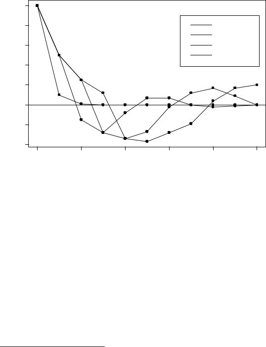
To illustrate the e ect of delay in the closed loop, consider the rst-order plant considered previously:
y[n + 1] = :5y[n] + :4u[n];
which decays geometrically to zero when the control signal u is zero, as shown earlier in Figure 3(a). Let us consider four closed-loop control laws with delays of zero, one, two, and three time steps respectively. With no delay, we set u[n] = ,Ky[n], and the closed loop becomes:
y[n + 1] = :5y[n] , :4Ky[n];
where K is the feedback gain. Letting K equal 1 yields the curve labelled T = 0 in Figure 10(a), where we see that the regulatory properties of the system are improved when compared to the open loop. If the plant output is
23
|
0.8 |
|
|
|
|
T = 0 |
|
|
|
|
|
T = 1 |
|
|
|
|
|
|
|
|
|
|
|
|
|
|
T = 2 |
|
0.4 |
|
|
|
|
T = 3 |
y[n] |
|
|
|
|
|
|
|
0.0 |
|
|
|
|
|
|
-0.4 |
|
|
|
|
|
|
0 |
2 |
4 |
6 |
8 |
10 |
|
|
|
|
n |
|
|
Figure 10: Performance of the feedback controller with delays in the feedback path.
delayed by one time step, we obtain u[n] = ,Ky[n , 1], and the closed-loop dynamics are given by
y[n + 1] = :5y[n] , :4Ky[n , 1];
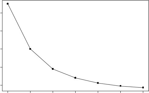
which is a second-order di erence equation. When K equals 1, the curve labelled T = 1 in Figure 10(b) is obtained, where we see that the delayed control signal has created an oscillation in the closed loop. As additional time steps of delay are introduced the closed loop becomes increasingly oscillatory and sluggish, as is shown by the curves labelled T = 2 and T = 3 in Figure 10(c). Eventually the closed-loop system becomes unstable. It is straightforward to solve for the maximum gain for which the closed loop remains stable at each value of delay.9 These values are plotted in Figure 11, where we see
9 These are the values of gain for which one of the roots of the characteristic equation of the closed-loop dynamics cross the unit circle in the complex plane (see, e.g., Astrom & Wittenmark, 1984).
24
|
3.5 |
gain |
3.0 |
maximum |
2.0 2.5 |
|
1.5 |
0 |
1 |
2 |
3 |
4 |
5 |
6 |
delay
Figure 11: Maximum possible gain for closed-loop stability as a function of feedback delay.
that the maximum permissible gain decreases as the delay increases. This plot illustrates a general point: To remain stable under conditions of delay, a closed-loop system must be operated at a lower feedback gain than a system without delay.
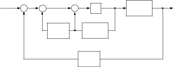
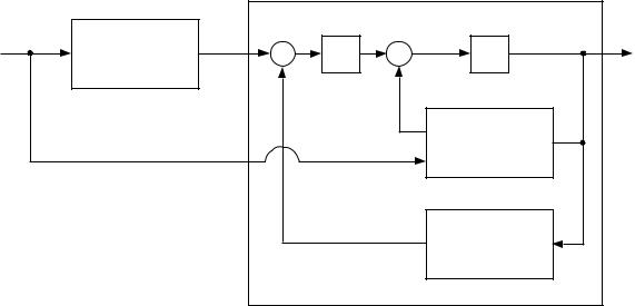
The Smith predictor
A general architecture for controlling a system with delay was developed by Smith (1958) and is referred to as a \Smith predictor." To understand the Smith predictor let us rst consider some simpler approaches to dealing with delay. The simplest scheme is to simply utilize an open-loop feedforward controller. If the feedforward controller is a reasonable approximation to an inverse of the plant then this scheme will control the plant successfully over short intervals of time. The inevitable disturbances and modeling errors will make performance degrade over longer time intervals, nonetheless, the advantages
25
of feedforward control are not to be neglected in this case. By ignoring the output from the plant, the feedforward system is stable in spite of the delay. It might be hoped that a feedforward controller could provide coarse control of the plant without compromising stability, thereby bringing the magnitude of the performance errors down to a level that could be handled by a low-gain feedback controller.
Composite feedforward and feedback control is indeed the idea behind the Smith predictor, but another issue arises due to the presence of delay. Let us suppose that the feedforward controller is a perfect inverse model of the plant and that there are no disturbances. In this case there should be no performance errors to correct. Note, however, that the performance error cannot be based on the di erence between the current reference signal and the current plant output, because the output of the plant is delayed by T time steps with respect to the reference signal. One approach to dealing with this problem would be to simply delay the reference signal by the appropriate amount before comparing it to the plant output. This approach has the disadvantage that the system is unable to anticipate potential future errors. Another approach|that used in the Smith predictor|is to utilize a forward model of the plant to predict the in uence of the feedforward control signal on the plant, delay this prediction by the appropriate amount, and add it to the control signal to cancel the anticipated contribution of the feedback controller.
The control system now has both an inverse model for control and a forward model for prediction. Recall that one way to implement a feedforward controller is to utilize a forward model in an internal feedback loop (cf. Figure 8). Thus a forward model can be used both for implementing the feedforward controller and for predicting the plant output. Placing the forward model in the forward path of the control system yields the Smith predictor, as shown in Figure 12. Note that if the forward model and the delay model in the Smith predictor are perfect, then the outer loop in the diagram is cancelled by the positive feedback loop that passes through the forward model and the delay model. The remaining loop (the negative feedback loop that passes through the forward model) is exactly the feedforward control scheme described previously in connection with Figure 8. Because this internal loop is not subject to delay from the periphery, the feedback gain K can be relatively large and the inner loop can therefore provide a reasonable approximation to an inverse plant model.
Although the intuitions behind the Smith predictor have been present in the motor control literature for many years, only recently has explicit use been made of this technique in motor control modeling. Miall, Weir, Wolpert and Stein (in press) have studied visuomotor tracking under conditions of varying
26
y*[n] + |
+ |
+ |
u[n] |
y[n] |
_ |
|
_ |
K |
Plant |
+ |
|
|
||
|
|
|
|
|
|
Delay |
|
Forward |
|
|
Model |
|
Model |
|
|
|
|
Delay |
|
Figure 12: The Smith predictor.
delay and have proposed a physiologically-based model of tracking in which the cerebellum acts as an adaptive Smith predictor.
Observers
In this section we brie y discuss the topic of state estimation. State estimation is a deep topic with rich connections to dynamical systems theory and statistical theory (Andersen & Moore, 1979). Our goal here is to simply provide some basic intuition for the problem, focusing on the important role of internal forward models in state estimation.
In the rst-order example that we have discussed, the problem of state estimation is trivial because the output of the system is the same as the state (Equation 13). In most situations the output is a more complex function of the state. In such situations it might be thought that the state could be recovered by simply inverting the output function. There are two fundamental reasons, however, why this is not a general solution to the problem of state estimation. First, there are usually more state variables than output variables in dynamical models, thus the function g is generally not uniquely invertible. An example is the one-joint robot arm considered earlier. The dynamical model of the arm has two state variables: the joint angle at the current time step and the joint angle at the previous time step. There is a single output variable: the current joint angle. Thus the output function preserves information about only one of the state variables, and it is impossible to recover the state by
27
|
|
|
Observer |
|
u[n] |
y[n ] |
+ |
+ |
^ |
x[n] |
||||
|
Plant |
_ |
K |
D |
|
|
+ |
|
|
|
|
|
|
|
|
|
|
|
Next-State |
|
|
|
|
Model |
|
|
|
|
Output |
|
|
|
|
Model |
Figure 13: An observer. The inputs to the observer are the plant input and output and the output from the observer is the estimated state of the plant.
simply inverting the output function. Minimally, the system must combine the outputs over two successive time steps in order to recover the state. The second reason why simply inverting the output function does not su ce is that in most situations there is stochastic uncertainty about the dynamics of the system as seen through its output. Such uncertainty may arise because of noise in the measurement device or because the dynamical system itself is a stochastic process. In either case, the only way to decrease the e ects of the uncertainty is to average across several nearby time steps.
The general conclusion that arises from these observations is that robust estimation of the state of a system requires observing the output of the system over an extended period of time. State estimation is fundamentally a dynamic process.
To provide some insight into the dynamical approach to state estimation, let us introduce the notion of an observer. As shown in Figure 13, an observer is a dynamical system that produces an estimate of the state of a system based on observations of the inputs and outputs of the system. The internal structure of an observer is intuitively very simple. The state of the observer is the variable x^[n], the estimate of the state of the plant. The observer has
28
access to the input to the plant, so it is in a position to predict the next state of the plant from the current input and its estimate of the current state. To make such a prediction the observer must have an internal model of the next-state function of the plant (the function f in Equation 1). If the internal model is accurate and if there is no noise in the measurement process or the state transition process, then the observer will accurately predict the next state of the plant. The observer is essentially an internal simulation of the plant dynamics that runs in parallel with the actual plant. Of course, errors will eventually accumulate in the internal simulation, thus there must be a way to couple the observer to the actual plant. This is achieved by using the plant output. Because the observer has access to the plant output, it is able to compare the plant output to its internal prediction of what the output should be, given its internal estimate of the state. To make such a prediction requires the observer to have an internal model of the output function of the plant (the function g in Equation 2). Errors in the observer's estimate of the state will be re ected in errors between the predicted plant output and the observed plant output. These errors can be used to correct the state estimate and thereby couple the observer dynamics to the plant dynamics.
The internal state of the observer evolves according to the following dynamical equation:
x^[n + 1] = f^(x^[n]; u[n]) + K(y[n] , g^(x^[n])); |
(23) |
where f^ and g^ are internal forward models of the next-state function and the output function, respectively. The rst term in the equation is the internal prediction of the next state of the plant, based on the current state estimate and the known input to the plant. The second term is the coupling term. It involves an error between the actual plant output and the internal prediction of the plant output. This error is multiplied by a gain K, known as the observer gain matrix. The weighted error is then added to the rst term to correct the state estimate.
In the case of linear dynamical systems, there is a well-developed theory to provide guidelines for setting the observer gain. In deterministic dynamical models, these guidelines provide conditions for maintaining the stability of the observer. Much stronger guidelines exist in the case of stochastic dynamical models, in which explicit assumptions are made about the probabilistic nature of the next-state function and the output function. In this case the observer is known as a \Kalman lter," and the observer gain is known as the \Kalman gain." The choice of the Kalman gain is based on the relative amount of noise in the next-state process and the output process. If there is relatively more noise in the output measurement process, then the observer should be
29
conservative in changing its internal state on the basis of the output error and thus the gain K should be small. Conversely, if there is relatively more noise in the state transition process, then the gain K should be large. An observer with large K averages the outputs over a larger span of time, which makes sense if the state transition dynamics are noisy. The Kalman lter quanti es these tradeo s and chooses the gain that provides an optimal tradeo between the two di erent kinds of noise. For further information on Kalman lters, see Anderson and Moore (1979).
In the case of nonlinear dynamical systems, the theory of state estimation is much less well-developed. Progress has been made, however, and the topic of the nonlinear observer is an active area of research (Misawa & Hedrick, 1989).
Learning Algorithms
In earlier sections we have seen several ways in which internal models can be used in a control system. Inverse models are the basic building block of feedforward control. Forward models can also be used in feedforward control, and have additional roles in state estimation and motor learning. It is important to emphasize that an internal model is a form of knowledge about the plant. Many motor control problems involve interacting with objects in the external world, and these objects generally have unknown mechanical properties. There are also changes in the musculoskeletal system due to growth or injury. These considerations suggest an important role for adaptive processes. Through adaptation the motor control system is able to maintain and update its internal models of external dynamics.
The next several sections develop some of the machinery that can be used to understand adaptive systems. Before entering into the details, let us rst establish some terminology and introduce a distinction. The adaptive algorithms that we will discuss are all instances of a general approach to learning known as error-correcting learning or supervised learning. A supervised learner is a system that learns a transformation from a set of inputs to a set of outputs. Examples of pairs of inputs and outputs are presented repeatedly to the learning system, and the system is required to abstract an underlying law or relation from this data so that it can generalize appropriately to new data. Within the general class of supervised learning algorithms, there are two basic classes of algorithms that it is useful to distinguish: regression algorithms and classi cation algorithms. A regression problem involves nding a functional relationship between the inputs and outputs. The form of the relationship
30