
Jordan M.Computational aspects of motor control and motor learning
.pdf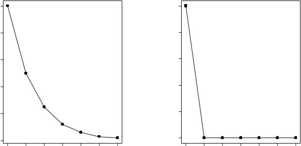
y[n] 0.0 0.2 0.4 0.6 0.8 1.0
|
|
|
|
|
(a) |
|
1.0 |
|
|
|
|
(b) |
|
|
|
|
|
|
|
|
|
|
|
|
|
||
|
|
|
|
|
|
|
0.8 |
|
|
|
|
|
|
|
|
|
|
|
|
|
0.6 |
|
|
|
|
|
|
|
|
|
|
|
|
|
y[n] |
|
|
|
|
|
|
|
|
|
|
|
|
|
0.4 |
|
|
|
|
|
|
|
|
|
|
|
|
|
0.2 |
|
|
|
|
|
|
|
|
|
|
|
|
|
0.0 |
|
|
|
|
|
|
0 |
1 |
2 |
3 |
4 |
5 |
6 |
0 |
1 |
2 |
3 |
4 |
5 |
6 |
|
|
|
n |
|
|
|
|
|
|
n |
|
|
|
Figure 3: (a) The output of the uncontrolled dynamical system in Equation 14
(a) (b)
with initial condition x[0] = 1. (b) The output of the dynamical system using the deadbeat controller in Equation 15. The desired output y [n] is xed at zero. The controller brings the actual output y[n] to zero in a single time step.
A predictive controller for this system can be obtained by solving for u[n] in Equation 14:
u[n] = ,1:25^x[n] + 2:5y [n + 1]: |
(15) |
Because this is an equation for a controller we treat y as the desired plant output rather than the actual plant output. Thus, the signal y [n + 1] is the input to the controller and denotes the desired future plant output. The controller output is u[n]. Note that we also assume that the state x[n] must be estimated.
Suppose that the controller has a good estimate of the state and suppose that it is desired to drive the output of the dynamical system to a value d as quickly as possible. Setting y [n + 1] to d, letting x^[n] equal x[n], and substituting Equation 15 into Equation 14, we see that indeed the output y at time n + 1 is equal to d (see Figure 3(b)). A predictive controller that can
11
y*[n+1] |
|
+ |
|
2.5
_
|
|
|
|
Plant |
|
u |
[ |
n |
+ |
y |
n |
|
] |
[ |
] |
||
|
|
|
.4 |
D |
|
|
|
|
+ |
|
|
|
|
|
|
.5 |
|
|
|
|
1.25 |
|
|
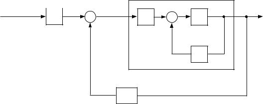
Figure 4: A deadbeat controller for the rst-order example.
drive the output of a dynamical system to an arbitrary desired value in k time steps, where k is the order of the dynamical system (i.e., the number of state variables), is referred to as a deadbeat controller. In the following section, we provide a further example of a deadbeat controller for a second-order system.
How should the state be estimated in the deadbeat controller? Because the output equation (Equation 13) shows that the state and the output are the same, a natural choice for the state estimate is the current output of the plant. Thus, the controller can be written in the more explicit form:
u[n] = ,1:25y[n] + 2:5y [n + 1]: |
(16) |
This choice of state estimator is not necessarily the best choice in the more realistic case in which there are disturbances acting on the system, however. In the section on observers, we shall discuss a more sophisticated approach to state estimation. Even in this more general framework, however, the state estimate is generally computed based on feedback from the output of the plant. Thus a deadbeat controller is generally a feedback controller. An alternative approach to predictive control design|open-loop feedforward control|is discussed below.
Figure 4 shows the deadbeat controller for the rst-order example. The symbol \D" in the gure refers to a one-time-step delay: A signal entering the delay is bu ered for one time step. That is, if the signal on the right-hand side of the delay is y[n], then the signal on the left-hand side of the delay is y[n+1]. It can be veri ed from the gure that y[n +1] is equal to the sum of :5y[n] and
12
:4u[n], as required by the dynamic equations for this system (Equations 14 and 13).
A second-order example
Higher-order dynamical systems are characterized by the property that the control signal does not normally have an immediate in uence on the output of the system, but rather exerts its in uence after a certain number of time steps, the number depending on the order of the system. In this section we design a deadbeat controller for a second-order plant to indicate how this issue can be addressed.
Consider a second-order dynamical system with the following next-state equation:
x1[n + 1] |
! = |
a1 a2 |
! |
x1[n] |
! + |
1 |
! u[n]; |
(17) |
x2[n + 1] |
1 0 |
x2[n] |
0 |
and output equation:
x [n] !
y[n] = 0 1 x1[n] : (18)
2
From the second row of Equation 17 it is clear that the control signal cannot a ect the second state variable in one time step. This implies, from Equation 18, that the control signal cannot a ect the output in a single time step. The control signal can a ect the output in two time steps, however. Therefore we attempt to obtain a predictive controller in which the control signal is a function of the desired output two time steps in the future. Extracting therst component of the next-state equation and solving for u[n] in terms of x2[n + 1], we obtain the following:
u[n] = ,a1x^1[n] , a2x^2[n] + y [n + 2]; |
(19) |
where we have used the fact that x1[n + 1] is equal to x2[n + 2] (from the second next-state equation) and x2[n + 2] is equal to y[n + 2] (from the output equation). Although this equation relates the control signal at time n to the desired output at time n + 2, there is a di culty in estimating the states. In particular, x1[n] is equal to y[n + 1], thus we would need access to a future value of the plant output in order to implement this controller. As it stands, the controller is unrealizable.
To remove the dependence on the future value of the output in Equation 19, let us substitute the next-state equation into itself, thereby replacing
13
x1[n] and x2[n] with x1[n , 1], x2[n , 1] and u[n , 1]. This substitution yields:
x1[n + 1] |
! = |
a12 + a2 a1a2 |
! |
x1[n , 1] |
!+ |
a1 |
! u[n,1]+ |
1 |
! u[n]: |
|
x2[n + 1] |
a1 |
a2 |
x2[n , 1] |
1 |
0 |
|||||
Extracting the rst component from this equation and solving for u[n] yields:
u[n] = ,(a12 + a2)^x1[n , 1] , a1a2x^2[n , 1] , a1u[n , 1] + y [n + 2]:
This equation depends only on quantities de ned at time n or earlier. In particular, x^1[n , 1] can be estimated by y[n] and x^2[n , 1] can be estimated by y[n , 1]. This yields the following deadbeat controller:
u[n] = ,(a12 + a2)y[n] , a1a2y[n , 1] , a1u[n , 1] + y [n + 2]: |
(20) |
The technique that we have described in this section is applicable to dynamical systems of any order. Because a state variable can always be expressed in terms of inputs and states at earlier moments in time, an unrealizable controller can always be converted into a realizable controller by expanding the next-state equation. It is also worth pointing out that the technique is also applicable to nonlinear systems, assuming that we are able to invert the equation relating the control signal to the future desired output signal. In cases in which this equation cannot be inverted analytically it may be possible to use numerical techniques.7 These issues will arise again in the section on motor learning.
Open-loop feedforward control
The second class of predictive control systems is the class of open-loop feedforward control systems. Like the deadbeat controller, the open-loop feedforward controller is based on an explicit inverse model of the plant. The logic behind the open-loop feedforward controller is the same as behind the deadbeat controller: The controller computes a control signal which is predicted to yield a desired future output. The di erence between the two approaches is the manner in which the state is estimated.
7 It is also worth raising a cautionary ag: There is an important class of systems, including some linear systems, for which the techniques that we are discussing do not su ce and must be extended. Some systems are uncontrollable, which means that there are state variables that cannot be a ected through a particular control variable. A proper treatment of this topic requires the notion of a controllability gramian. For further discussion, see Astrom & Wittenmark (1984).
14

|
|
|
|
|
|
Plant |
|
|
* |
|
u |
|
n |
|
y |
n |
|
y [n+1] |
+ |
[ |
+ |
|||||
|
] |
[ |
] |
|||||
2.5 |
_ |
|
|
|
.4 |
D |
|
|
|
|
|
|
+ |
|
|
||
|
|
|
|
|
|
|
||
D |
1.25 |
|
|
|
|
.5 |
|
Figure 5: An open-loop feedforward controller for the rst-order example.
Example
In the previous section, we saw that a deadbeat controller for the rstorder plant has the form:
u[n] = ,1:25y[n] + 2:5y [n + 1];
where the signal y[n] is considered to be an estimate of the state of the plant. We might also consider a controller of the following form:
u[n] = ,1:25y [n] + 2:5y [n + 1]; |
(21) |
in which the state is estimated by the desired plant output y [n] rather than the actual plant output y[n]. Figure 5 shows a diagrammatic representation of this controller. Note that there is no feedback from the plant to the controller; the loop from plant to controller has been \opened." Because of the lack of a feedback term in the control equation, the open-loop approach allows the entire control signal to be \preprogrammed" if the desired output trajectory is known in advance. The justi cation for the open-loop approach is that a good controller will keep the actual output and the desired output close together, so that replacing y[n] by y [n] in estimating the state may not incur much error. This is a strong assumption, however, because there are many sources of inaccuracy that can degrade the performance of a feedforward controller. In particular, if there are disturbances acting on the plant, then the state of the plant will diverge from the internal estimate of the state. Of course, no controller can control a system perfectly in the presence of disturbances. A system that utilizes feedback, however, has its state estimate continually reset and is therefore less likely to diverge signi cantly from reality than an openloop controller. Another source of error is that the controller itself may be an
15
inaccurate inverse model of the plant. Feedback renders the control system less sensitive to such inaccuracies.
One disadvantage of controllers based on feedback is that feedback can introduce stability problems. For this reason, open-loop feedforward controllers have important roles to play in certain kinds of control problems. As we discuss in a later section, stability is particularly of concern in systems with delay in the feedback pathway, thus an open-loop controller may be a reasonable option in such cases. Open-loop controllers also have an important role to play in composite control systems, when they are combined with an error-correcting feedback controller (see below). The division of labor into open-loop control and error-correcting control can be a useful way of of organizing complex control tasks.
Biological examples of feedforward control
There are many examples of open-loop feedforward control systems in the motor control literature. A particularly clear example is the vestibulo-ocular re ex (VOR). The VOR couples the movement of the eyes to the motion of the head, thereby allowing an organism to keep its gaze xed in space. This is achieved by causing the the motion of the eyes to be equal and opposite to the motion of the head. The VOR control system is typically modeled as a transformation from head velocity to eye velocity (Robinson, 1981). The head velocity signal, provided by the vestibular system, is fed to a control system that provides neural input to the eye muscles. In our notation, the head velocity signal is the controller input ,y [n], the neural command to the muscles is the control signal u[n], and the eye velocity signal is the plant output y[n]. Note that the plant output (the eye velocity) has no e ect on the control input (the head motion), thus the VOR is an open-loop feedforward control system. This implies that the neural machinery must implement an open-loop inverse model of the oculomotor plant. It is generally agreed in the literature on the VOR that such an inverse model exists in the neural circuitry and there have been two principal proposals for the neural implementation of the inverse model. Robinson (1981) has proposed a model based on an open-loop feedforward controller of the form shown earlier in Figure 5. In this model, as in the gure, the inverse model is implemented by adding the signals on a pair of parallel channels: a feed-through pathway and a pathway incorporating a delay (which corresponds to an integrator in Robinson's continuous-time model). An alternative model, proposed by Galliana and Outerbridge (1984), implements the inverse model by placing a forward model of the plant in an internal feedback pathway. (A closely related technique is described below;
16
see Figure 8).
Another interesting example of feedforward control arises in the literature on speech production. Lindblom, Lubker and Gay (1979) studied an experimental task in which subjects produced vowel sounds while their jaw was held open by a bite block. Lindblom et al. observed that the vowels produced by the subjects had formant frequencies in the normal range, despite the fact that unusual articulatory postures were required to produce these sounds. Moreover, the formant frequencies were in the normal range during the rst pitch period, before any possible in uence of acoustic feedback. This implies feedforward control of articulatory posture (with respect to the acoustic goal). Lindblom et al. proposed a qualitative model of this feedforward control system that again involved placing a forward model of the plant in an internal feedback pathway (see Figure 8).
Error-correcting feedback control
In this section we provide a brief overview of error-correcting feedback control systems. Error-correcting feedback control di ers from predictive control in that it does not rely on an explicit inverse model of the plant. As we shall see, however, an error-correcting feedback control system can be thought of as implicitly computing an approximate plant inverse; thus, these two forms of control are not as distinct as they may seem.
An error-correcting feedback controller works directly to correct the error at the current time step between the desired output and the actual output. Consider the rst order system presented earlier. A natural choice for an error-correcting feedback signal would be the weighted error:
u[n] = K(y [n] , y[n]); |
(22) |
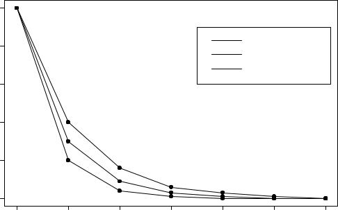
where the scalar K is referred to as a gain. Note that the reference signal for this controller is the current desired output (y [n]) rather than the future desired output (y [n + 1]) as in the predictive control approach. The performance of this feedback controller is shown in Figure 6 for several values of K. As K increases, the feedback controller brings the output of the plant to the desired value more rapidly.
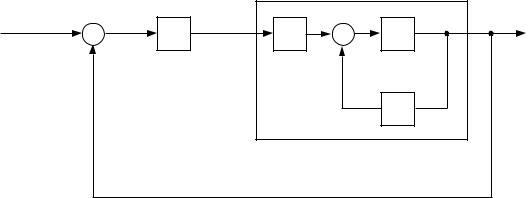
A block diagram of the error-correctin feedback control system is shown in Figure 7, to be compared to the predictive controllers in Figure 4 and Figure 5. Several general distinctions can be drawn from comparing these control systems. One important distinction between predictive and error-correcting control is based on the temporal relationships that are involved. In predictive control, the control signal is a function of the future desired output. If the
17
|
1.0 |
|
|
|
|
|
|
|
0.8 |
|
|
|
|
K = 0.25 |
|
|
|
|
|
|
K = 0.5 |
|
|
|
|
|
|
|
|
|
|
|
0.4 0.6 |
|
|
|
|
K = 0.75 |
|
y[n] |
|
|
|
|
|
|
|
|
0.2 |
|
|
|
|
|
|
|
0.0 |
|
|
|
|
|
|
|
0 |
1 |
2 |
3 |
4 |
5 |
6 |
|
|
|
|
n |
|
|
|
Figure 6: Performance of the error-correcting feedback controller as a function of the gain. The desired output y [n] is xed at zero.
predictive controller is a perfect inverse model of the plant, and if there are no unmodeled disturbances acting on the plant, then the future desired output will indeed be achieved by using the computed control signal. That is, an ideal predictive controller operates without error. An error-correcting feedback controller, on the other hand, corrects the error after the error has occurred, thus even under ideal conditions such a controller exhibits a certain amount of error. The assumption underlying error-correcting control is that the desired output changes relatively slowly; thus, correcting the error at the current time step is likely to diminish the error at the following time step as well. Another distinction between predictive control and error-correcting control has to do with the role of explicit knowledge about the plant. Predictive control requires explicit knowledge of the dynamics of the plant (a predictive controller is an inverse model of the plant). For example, the coe cients 1.25 and 2.5 in the predictive controllers in the previous section are obtained explicitly from knowledge of the coe cients of the plant dynamic equation. Error-correcting control does
18
|
|
|
|
|
|
Plant |
|
y* n |
+ |
u |
[ |
n |
+ |
y |
n |
[ ] |
|
] |
[ |
] |
|||
|
K |
|
|
|
.4 |
D |
|
|
_ |
|
|
|
+ |
|
|
|
|
|
|
|
|
|
|
|
|
|
|
|
|
.5 |
|
Figure 7: An error-correcting feedback controller for the rst-order example.
not require the implementation of an explicit plant model. The design of an error-correcting controller (i.e., the choice of the feedback gain) generally depends on knowledge of the plant. However the knowledge that is required for such control design is often rather qualitative. Moreover, the performance of an error-correcting controller is generally rather insensitive to the exact value of the gain that is chosen. The predictive controllers based on feedback (i.e., the deadbeat controllers) are also somewhat insensitive to the exact values of their coe cients. This is in contrast to open-loop controllers, for which the performance is generally highly sensitive to the values of the coe cients. For example, choosing a value other than 2.5 in the forward path of the open-loop controller in the previous section yields a steady-state error at the output of the plant. Finally, as we have stated earlier, feedback controllers tend to be more robust to unanticipated disturbances than open-loop controllers.
Feedback control and plant inversion
Let us now establish a relationship between error-correcting feedback control and the notion of inverting a dynamical system. To simplify the argument we restrict ourselves to the rst-order plant considered previously (Figure 7). Consider now the system shown in Figure 8, in which a replica of the plant is placed in a feedback path from the control signal to the error signal. This system is entirely equivalent to the preceding system, if we assume that there are no disturbances acting at the output of the plant. That is, the control
19
|
|
|
|
|
|
|
|
|
|
|
Plant |
|
y*[n] + |
|
|
|
|
|
|
|
u[n] |
|
|
y[n] |
|
|
|
|
|
|
|
|
|
|
||||
|
|
|
|
K |
|
|
||||||
|
_ |
|
|
|
|
|
|
|
|
|
|
|
|
|
|
|
|
|
|
|
|
|
|
||
|
|
|
Plant |
|
|
|
|
|||||
y[n] |
|
|
|
|
|
|
|
|||||
|
|
|
|
|
|
|
||||||
|
|
|
|
|
|
|
|
|
|
|
|
|
|
|
|
|
|
|
|
|
|
|
|
|
|
|
|
|
|
|
|
|
|
|
|
|
|
|
Figure 8: A control system in which the control signal is fed back through a replica of the plant. This system is mathematically equivalent to the feedback control system shown in Figure 7.
signal in both diagrams is exactly the same:
u[n] = K(y [n] , y[n]):
This error equation can be expanded using the next-state equation (Equation 12) and the output equation (Equation 13):
u[n] = Ky [n] , :5Ky[n , 1] , :4Ku[n , 1]:
Dividing by K and moving u[n , 1] to the left-hand side yields:
K1 u[n] + :4u[n , 1] = y [n] , :5y[n , 1]:
If we now let the gain K go to in nity, the rst term drops away, and we are left with an expression for u[n , 1]:
:4u[n , 1] = y [n] , :5y[n , 1]:
Shifting the time index and rearranging yields:
u[n] = ,1:25y[n] + 2:5y [n + 1]:
This expression is an inverse dynamic model of the plant (cf. Equation 16). What we have shown is that for large values of the gain, the internal loop
in Figure 8 computes approximately the same control signal as an explicit
20
