page 266

y

P = ( x, y, z)

y

z x

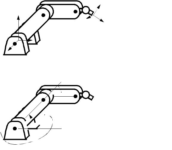
Tool Coordinates - here the tool orientation is considered, and

x

the coordinates are measured against a frame attached to the tool

z

Figure 7.4 - Tool Coordinates - Describing Positions Relative to the Tool

θ 3

θ 2 θ 1

Joint Coordinates - the position of each joint (all angles here) are used to describe the position of the robot.

Figure 7.5 - Joint Coordinates - the Positions of the Actuators

9.1.2 Positioning Concepts

9.1.2.1 - Accuracy and Repeatability

•The accuracy and repeatability are functions of,

-resolutionthe use of digital systems, and other factors mean that only a limited number of positions are available. Thus user input coordinates are often adjusted to the nearest discrete position.

-kinematic modeling error - the kinematic model of the robot does not exactly match the

page 267

robot. As a result the calculations of required joint angles contain a small error.

-calibration errors - The position determined during calibration may be off slightly, resulting in an error in calculated position.

-random errors - problems arise as the robot operates. For example, friction, structural bending, thermal expansion, backlash/slip in transmissions, etc. can cause variations in position.

•Accuracy,

•“How close does the robot get to the desired point”

•This measures the distance between the specified position, and the actual position of the robot end effector.

•Accuracy is more important when performing off-line programming, because absolute coordinates are used.

•Repeatability

•“How close will the robot be to the same position as the same move made before”

•A measure of the error or variability when repeatedly reaching for a single position.

•This is the result of random errors only

•repeatability is often smaller than accuracy.

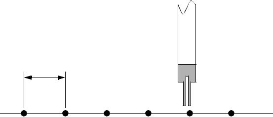
•Resolution is based on a limited number of points that the robot can be commanded to reach for, these are shown here as black dots. These points are typically separated by a millimeter or less, depending on the type of robot. This is further complicated by the fact that the user might ask for a position such as 456.4mm, and the system can only move to the nearest millimeter, 456mm, this is the accuracy error of 0.4mm.

R

page 268

• In a perfect mechanical situation the accuracy and control resolution would be determined

as below,

The manipulator may stop at a number of discrete positions

One axis on a surface

control resolution

specified locations

In an ideal situation the manipulator would stop at the specified locations. Here the accuracy would be half of the control resolution. The control resolution would be the smallest divisions that the workspace could be divided into (often by the resolution of digital components.

• Kinematic and calibration errors basically shift the points in the workspace resulting in an

error ‘e’. Typically vendor specifications assume that calibration and modeling errors are zero.

page 269

error ‘e’

Should be here

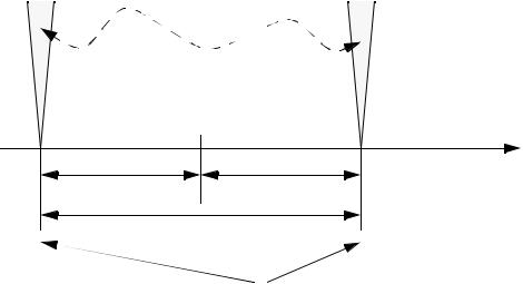
• Random errors will prevent the robot from returning to the exact same location each time,

and this can be shown with a probability distribution about each point.

System specified

position ‘S’

User requested position ‘U’

accuracy ‘a/2’

If the distribution is normal, the limits for repeatability are typically chosen as ±3 standard deviations ‘s’.