

page 576
cov = ∑ ( xi – µ x) ( yi – µ y) – µ xµ y |
corr = |
|
cov |
----------- |
|||
|
|
σ |
xσ y |
where,
cov = covariance of data sets x and y corr = correllation of sets x and y
corr = 1 completely related corr = 0 no relationship corr = -1 inversely related
•Simulation software will provide information such as,
-production rates
-machine usage
-buffer size
-work in process
22.3 DESIGN OF EXPERIMENTS
•WHAT? combinations of individual parameters for process control are varied, and their effect on the output quality are measured. From this we determine the sensitivity of the process to each parameter.
•WHY? Because randomly varying individual parameters takes too long.
•e.g. A One-Factor-At-A-Time-Experiment

page 577
Effect: We are finding the causes of cracks in steel springs.
Causes:
1.Steel temperature before quenching 1450F or 1600F
2.Carbon Content .5% or .7%
3.Oil quench temperature 70F or 50F
Experiments 1 and 2: Run 1:
1. 1450F 
2. 0.5% yield(%) 72 70 75 77, X=73.5%
3. 70F 
Run 2:
1. **1600F
2. 0.5% yield(%) 78 77 78 81, X=78.5%
3. 70F 
Observation: 1600F before quench gives higher yield.
Run 3:
1. 1600F
2. **0.7%
3. 70F 
Observation: Adding more carbon has a small negative effect on yield.
Run 4:
1. 1600F
2. 0.5% yield(%) 79 78 78 83, X=79.5%
3. **50F
Observation: We have improved the quality by 6%, but it has required 4 runs, and we could continue.
•The example shows how the number of samples grows quickly.
•A better approach is designed experiments
•e.g. DESIGNED EXPERIMENT for springs in last section
page 578
- set up orthogonal array |
|
|
|
|
|
|
|
||||
Run |
|
1. |
2. |
3. |
|
Yield% |
|
Ri = |
|
|
|
X |
|||||||||||
|
|
|
|
||||||||
|
|
|
|
|
|
|
|
|
|
|
|
1 |
|
1450 |
0.5 |
50 |
|
|
|
|
|
|
|
2 |
|
1600 |
0.5 |
50 |
|
79 78 78 83 |
|
79.5 |
|
|
|
3 |
|
1450 |
0.7 |
50 |
|
|
|
|
|
|
|
4 |
|
1600 |
0.7 |
50 |
|
|
|
|
|
|
|
5 |
|
1450 |
0.5 |
70 |
|
72 70 75 77 |
|
73.5 |
|
|
|
6 |
|
1600 |
0.5 |
70 |
|
78 77 78 81 |
|
78.5 |
|
|
|
7 |
|
1450 |
0.7 |
70 |
|
|
|
|
|
|
|
8 |
|
1600 |
0.7 |
70 |
|
77 78 75 80 |
|
77.5 |
|
|
|
Note the binary sequence
- Find effects of each factor
Main Effect = ( Average at High) – ( Average at Low)
Main Effect of A = |
(-----------------------------------------------R2 + R4 + R6 + R8) |
– |
(-----------------------------------------------R1 + R3 + R5 + R7) |
|
4 |
|
4 |
Main Effect of B = |
(-----------------------------------------------R1 + R2 + R5 + R6) |
– |
(-----------------------------------------------R3 + R4 + R7 + R8) |
|
4 |
|
4 |
Main Effect of C = |
(-----------------------------------------------R1 + R2 + R3 + R4) |
– |
(-----------------------------------------------R5 + R6 + R7 + R8) |
|
4 |
|
4 |
- these can be drawn on an effect graph
Yield
%
A- |
A+ |
B- |
B+ |
C- |
C+ |
page 579
22.4 RUNNING THE SIMULATION
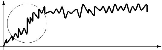
• When a simulation is first run it will be empty. If it is allowed to run for a while it will settle
down to a steady state. We will typically want to,
-run the simulation for a long time
-or, delay the start of data collection
-or, preload the system will parts
Problem area |
22.5 DECISION MAKING STRATEGY
•The general sequence of thought when making decisions is,
-purpose
-direction
-plans
-action
-results
•General properties of strategy include,
-time horizon
-impact
-concentration of effort
-patterns of decisions
page 580
-pervasiveness
•The levels of strategies include,
-corporate
-business
-departmental/functional
•Decisions can be categorized, hardware/fixed
-capacity
-facilities
-technology
-vertical integration software/flexible
-workforce
-quality
-production planning/material control
-organization
•Typical criteria for making decisions might include,
-consistency
-harmony
-contribution