page 262

9. INDUSTRIAL ROBOTICS

9.1 INTRODUCTION

Robots are devices that are programmed to move parts, or to do work with a tool. For exam-

ple, robots are often used to stack boxes on a pallet, or to weld steel plates together. This chapter

will introduce the basic concepts behind robotics, and introduce a commercial robot. Following

chapters will introduce more robots, and discuss applications.

9.1.1 Basic Terms

There is a set of basic terminology and concepts common to all robots. These terms follow

with brief explanations of each.

Links and Joints - Links are the solid structural members of a robot, and joints are the movable couplings between them.

Degree of Freedom (dof) - Each joint on the robot introduces a degree of freedom. Each dof can be a slider, rotary, or other type of actuator. Robots typically have 5 or 6 degrees of freedom. 3 of the degrees of freedom allow positioning in 3D space, while the other 2or 3 are used for orientation of the end effector. 6 degrees of freedom are enough to allow the robot to reach all positions and orientations in 3D space. 5 dof requires a restriction to 2D space, or else it limits orientations. 5 dof robots are commonly used for handling tools such as arc welders.

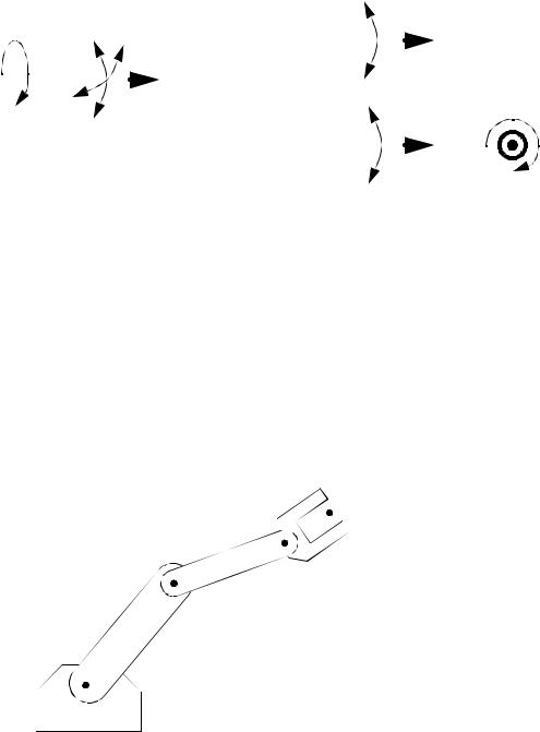
Orientation Axes - Basically, if the tool is held at a fixed position, the orientation determines which direction it can be pointed in. Roll, pitch and yaw are the common orientation axes used. Looking at the figure below it will be obvious that the tool can be positioned at any orientation in space. (imagine sitting in a plane. If the plane rolls you will turn upside down. The pitch changes for takeoff and landing and when flying in a crosswind the plane will yaw.)

page 263

Position Axes - The tool, regardless of orientation, can be moved to a number of positions in space. Various robot geometries are suited to different work geometries. (more later)

Tool Centre Point (TCP) - The tool centre point is located either on the robot, or the tool. Typically the TCP is used when referring to the robots position, as well as the focal point of the tool. (e.g. the TCP could be at the tip of a welding torch) The TCP can be specified in cartesian, cylindrical, spherical, etc. coordinates depending on the robot. As tools are changed we will often reprogram the robot for the TCP.

TCP

(Tool Center Point)

Figure 7.2 - The Tool Center Point (TCP)

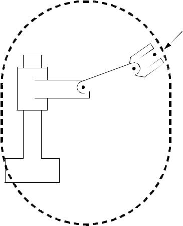
Work envelope/Workspace - The robot tends to have a fixed, and limited geometry. The work envelope is the boundary of positions in space that the robot can reach. For a cartesian robot (like an overhead crane) the workspace might be a square, for more sophisticated robots the workspace might be a shape that looks like a ‘clump of intersecting bubbles’.

page 264

Workspace

Speed - refers either to the maximum velocity that is achievable by the TCP, or by individual joints. This number is not accurate in most robots, and will vary over the workspace as the geometry of the robot changes (and hence the dynamic effects). The number will often reflect the maximum safest speed possible. Some robots allow the maximum rated speed (100%) to be passed, but it should be done with great care.

Payload - The payload indicates the maximum mass the robot can lift before either failure of the robots, or dramatic loss of accuracy. It is possible to exceed the maximum payload, and still have the robot operate, but this is not advised. When the robot is accelerating fast, the payload should be less than the maximum mass. This is affected by the ability to firmly grip the part, as well as the robot structure, and the actuators. The end of arm tooling should be considered part of the payload.

Repeatability - The robot mechanism will have some natural variance in it. This means that when the robot is repeatedly instructed to return to the same point, it will not always stop at the same position. Repeatability is considered to be +/-3 times the

page 265

standard deviation of the position, or where 99.5% of all repeatability measurements fall. This figure will vary over the workspace, especially near the boundaries of the workspace, but manufacturers will give a single value in specifications.

Accuracy - This is determined by the resolution of the workspace. If the robot is commanded to travel to a point in space, it will often be off by some amount, the maximum distance should be considered the accuracy. This is an effect of a control system that is not necessarily continuous.

Settling Time - During a movement, the robot moves fast, but as the robot approaches the final position is slows down, and slowly approaches. The settling time is the time required for the robot to be within a given distance from the final position.

Control Resolution - This is the smallest change that can be measured by the feedback sensors, or caused by the actuators, whichever is larger. If a rotary joint has an encoder that measures every 0.01 degree of rotation, and a direct drive servo motor is used to drive the joint, with a resolution of 0.5 degrees, then the control resolution is about 0.5 degrees (the worst case can be 0.5+0.01).

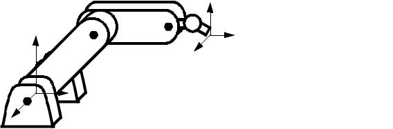
Coordinates - The robot can move, therefore it is necessary to define positions. Note that coordinates are a combination of both the position of the origin and orientation of the axes.

y

P = ( x, y, z)

y

x

z

World Coordinates - this is the position of the tool measured

x

relative to the base, the orientation of the tool is assumed to be the same as the base.

z

Figure 7.3 - World Coordinates - To Locate the TCP