
- •1. INTEGRATED AND AUTOMATED MANUFACTURING
- •1.1 INTRODUCTION
- •1.1.1 Why Integrate?
- •1.1.2 Why Automate?
- •1.2 THE BIG PICTURE
- •1.2.2 The Architecture of Integration
- •1.2.3 General Concepts
- •1.3 PRACTICE PROBLEMS
- •2. AN INTRODUCTION TO LINUX/UNIX
- •2.1 OVERVIEW
- •2.1.1 What is it?
- •2.1.2 A (Brief) History
- •2.1.3 Hardware required and supported
- •2.1.4 Applications and uses
- •2.1.5 Advantages and Disadvantages
- •2.1.6 Getting It
- •2.1.7 Distributions
- •2.1.8 Installing
- •2.2 USING LINUX
- •2.2.1 Some Terminology
- •2.2.2 File and directories
- •2.2.3 User accounts and root
- •2.2.4 Processes
- •2.3 NETWORKING
- •2.3.1 Security
- •2.4 INTERMEDIATE CONCEPTS
- •2.4.1 Shells
- •2.4.2 X-Windows
- •2.4.3 Configuring
- •2.4.4 Desktop Tools
- •2.5 LABORATORY - A LINUX SERVER
- •2.6 TUTORIAL - INSTALLING LINUX
- •2.7 TUTORIAL - USING LINUX
- •2.8 REFERENCES
- •3. AN INTRODUCTION TO C/C++ PROGRAMMING
- •3.1 INTRODUCTION
- •3.2 PROGRAM PARTS
- •3.3 CLASSES AND OVERLOADING
- •3.4 HOW A ‘C’ COMPILER WORKS
- •3.5 STRUCTURED ‘C’ CODE
- •3.6 COMPILING C PROGRAMS IN LINUX
- •3.6.1 Makefiles
- •3.7 ARCHITECTURE OF ‘C’ PROGRAMS (TOP-DOWN)
- •3.8 CREATING TOP DOWN PROGRAMS
- •3.9 CASE STUDY - THE BEAMCAD PROGRAM
- •3.9.1 Objectives:
- •3.9.2 Problem Definition:
- •3.9.3 User Interface:
- •3.9.3.1 - Screen Layout (also see figure):
- •3.9.3.2 - Input:
- •3.9.3.3 - Output:
- •3.9.3.4 - Help:
- •3.9.3.5 - Error Checking:
- •3.9.3.6 - Miscellaneous:
- •3.9.4 Flow Program:
- •3.9.5 Expand Program:
- •3.9.6 Testing and Debugging:
- •3.9.7 Documentation
- •3.9.7.1 - Users Manual:
- •3.9.7.2 - Programmers Manual:
- •3.9.8 Listing of BeamCAD Program.
- •3.10 PRACTICE PROBLEMS
- •3.11 LABORATORY - C PROGRAMMING
- •4. NETWORK COMMUNICATION
- •4.1 INTRODUCTION
- •4.2 NETWORKS
- •4.2.1 Topology
- •4.2.2 OSI Network Model
- •4.2.3 Networking Hardware
- •4.2.4 Control Network Issues
- •4.2.5 Ethernet
- •4.2.6 SLIP and PPP
- •4.3 INTERNET
- •4.3.1 Computer Addresses
- •4.3.2 Computer Ports
- •4.3.2.1 - Mail Transfer Protocols
- •4.3.2.2 - FTP - File Transfer Protocol
- •4.3.2.3 - HTTP - Hypertext Transfer Protocol
- •4.3.3 Security
- •4.3.3.1 - Firewalls and IP Masquerading
- •4.4 FORMATS
- •4.4.1 HTML
- •4.4.2 URLs
- •4.4.3 Encryption
- •4.4.4 Clients and Servers
- •4.4.5 Java
- •4.4.6 Javascript
- •4.5 NETWORKING IN LINUX
- •4.5.1 Network Programming in Linux
- •4.6 DESIGN CASES
- •4.7 SUMMARY
- •4.8 PRACTICE PROBLEMS
- •4.9 LABORATORY - NETWORKING
- •4.9.1 Prelab
- •4.9.2 Laboratory
- •5. DATABASES
- •5.1 SQL AND RELATIONAL DATABASES
- •5.2 DATABASE ISSUES
- •5.3 LABORATORY - SQL FOR DATABASE INTEGRATION
- •5.4 LABORATORY - USING C FOR DATABASE CALLS
- •6. COMMUNICATIONS
- •6.1 SERIAL COMMUNICATIONS
- •6.2 SERIAL COMMUNICATIONS UNDER LINUX
- •6.3 PARALLEL COMMUNICATIONS
- •6.4 LABORATORY - SERIAL INTERFACING AND PROGRAMMING
- •6.5 LABORATORY - STEPPER MOTOR CONTROLLER
- •7. PROGRAMMABLE LOGIC CONTROLLERS (PLCs)
- •7.1 BASIC LADDER LOGIC
- •7.2 WHAT DOES LADDER LOGIC DO?
- •7.2.1 Connecting A PLC To A Process
- •7.2.2 PLC Operation
- •7.3 LADDER LOGIC
- •7.3.1 Relay Terminology
- •7.3.2 Ladder Logic Inputs
- •7.3.3 Ladder Logic Outputs
- •7.4 LADDER DIAGRAMS
- •7.4.1 Ladder Logic Design
- •7.4.2 A More Complicated Example of Design
- •7.5 TIMERS/COUNTERS/LATCHES
- •7.6 LATCHES
- •7.7 TIMERS
- •7.8 COUNTERS
- •7.9 DESIGN AND SAFETY
- •7.9.1 FLOW CHARTS
- •7.10 SAFETY
- •7.10.1 Grounding
- •7.10.2 Programming/Wiring
- •7.10.3 PLC Safety Rules
- •7.10.4 Troubleshooting
- •7.11 DESIGN CASES
- •7.11.1 DEADMAN SWITCH
- •7.11.2 CONVEYOR
- •7.11.3 ACCEPT/REJECT SORTING
- •7.11.4 SHEAR PRESS
- •7.12 ADDRESSING
- •7.12.1 Data Files
- •7.12.1.1 - Inputs and Outputs
- •7.12.1.2 - User Numerical Memory
- •7.12.1.3 - Timer Counter Memory
- •7.12.1.4 - PLC Status Bits (for PLC-5s)
- •7.12.1.5 - User Function Memory
- •7.13 INSTRUCTION TYPES
- •7.13.1 Program Control Structures
- •7.13.2 Branching and Looping
- •7.13.2.1 - Immediate I/O Instructions
- •7.13.2.2 - Fault Detection and Interrupts
- •7.13.3 Basic Data Handling
- •7.13.3.1 - Move Functions
- •7.14 MATH FUNCTIONS
- •7.15 LOGICAL FUNCTIONS
- •7.15.1 Comparison of Values
- •7.16 BINARY FUNCTIONS
- •7.17 ADVANCED DATA HANDLING
- •7.17.1 Multiple Data Value Functions
- •7.17.2 Block Transfer Functions
- •7.18 COMPLEX FUNCTIONS
- •7.18.1 Shift Registers
- •7.18.2 Stacks
- •7.18.3 Sequencers
- •7.19 ASCII FUNCTIONS
- •7.20 DESIGN TECHNIQUES
- •7.20.1 State Diagrams
- •7.21 DESIGN CASES
- •7.21.1 If-Then
- •7.21.2 For-Next
- •7.21.3 Conveyor
- •7.22 IMPLEMENTATION
- •7.23 PLC WIRING
- •7.23.1 SWITCHED INPUTS AND OUTPUTS
- •7.23.1.1 - Input Modules
- •7.23.1.2 - Actuators
- •7.23.1.3 - Output Modules
- •7.24 THE PLC ENVIRONMENT
- •7.24.1 Electrical Wiring Diagrams
- •7.24.2 Wiring
- •7.24.3 Shielding and Grounding
- •7.24.4 PLC Environment
- •7.24.5 SPECIAL I/O MODULES
- •7.25 PRACTICE PROBLEMS
- •7.26 REFERENCES
- •7.27 LABORATORY - SERIAL INTERFACING TO A PLC
- •8. PLCS AND NETWORKING
- •8.1 OPEN NETWORK TYPES
- •8.1.1 Devicenet
- •8.1.2 CANbus
- •8.1.3 Controlnet
- •8.1.4 Profibus
- •8.2 PROPRIETARY NETWORKS
- •8.2.0.1 - Data Highway
- •8.3 PRACTICE PROBLEMS
- •8.4 LABORATORY - DEVICENET
- •8.5 TUTORIAL - SOFTPLC AND DEVICENET
- •9. INDUSTRIAL ROBOTICS
- •9.1 INTRODUCTION
- •9.1.1 Basic Terms
- •9.1.2 Positioning Concepts
- •9.1.2.1 - Accuracy and Repeatability
- •9.1.2.2 - Control Resolution
- •9.1.2.3 - Payload
- •9.2 ROBOT TYPES
- •9.2.1 Basic Robotic Systems
- •9.2.2 Types of Robots
- •9.2.2.1 - Robotic Arms
- •9.2.2.2 - Autonomous/Mobile Robots
- •9.2.2.2.1 - Automatic Guided Vehicles (AGVs)
- •9.3 MECHANISMS
- •9.4 ACTUATORS
- •9.5 A COMMERCIAL ROBOT
- •9.5.1 Mitsubishi RV-M1 Manipulator
- •9.5.2 Movemaster Programs
- •9.5.2.0.1 - Language Examples
- •9.5.3 Command Summary
- •9.6 PRACTICE PROBLEMS
- •9.7 LABORATORY - MITSUBISHI RV-M1 ROBOT
- •9.8 TUTORIAL - MITSUBISHI RV-M1
- •10. OTHER INDUSTRIAL ROBOTS
- •10.1 SEIKO RT 3000 MANIPULATOR
- •10.1.1 DARL Programs
- •10.1.1.1 - Language Examples
- •10.1.1.2 - Commands Summary
- •10.2 IBM 7535 MANIPULATOR
- •10.2.1 AML Programs
- •10.3 ASEA IRB-1000
- •10.4 UNIMATION PUMA (360, 550, 560 SERIES)
- •10.5 PRACTICE PROBLEMS
- •10.6 LABORATORY - SEIKO RT-3000 ROBOT
- •10.7 TUTORIAL - SEIKO RT-3000 ROBOT
- •10.8 LABORATORY - ASEA IRB-1000 ROBOT
- •10.9 TUTORIAL - ASEA IRB-1000 ROBOT
- •11. ROBOT APPLICATIONS
- •11.0.1 Overview
- •11.0.2 Spray Painting and Finishing
- •11.0.3 Welding
- •11.0.4 Assembly
- •11.0.5 Belt Based Material Transfer
- •11.1 END OF ARM TOOLING (EOAT)
- •11.1.1 EOAT Design
- •11.1.2 Gripper Mechanisms
- •11.1.2.1 - Vacuum grippers
- •11.1.3 Magnetic Grippers
- •11.1.3.1 - Adhesive Grippers
- •11.1.4 Expanding Grippers
- •11.1.5 Other Types Of Grippers
- •11.2 ADVANCED TOPICS
- •11.2.1 Simulation/Off-line Programming
- •11.3 INTERFACING
- •11.4 PRACTICE PROBLEMS
- •11.5 LABORATORY - ROBOT INTERFACING
- •11.6 LABORATORY - ROBOT WORKCELL INTEGRATION
- •12. SPATIAL KINEMATICS
- •12.1 BASICS
- •12.1.1 Degrees of Freedom
- •12.2 HOMOGENEOUS MATRICES
- •12.2.1 Denavit-Hartenberg Transformation (D-H)
- •12.2.2 Orientation
- •12.2.3 Inverse Kinematics
- •12.2.4 The Jacobian
- •12.3 SPATIAL DYNAMICS
- •12.3.1 Moments of Inertia About Arbitrary Axes
- •12.3.2 Euler’s Equations of Motion
- •12.3.3 Impulses and Momentum
- •12.3.3.1 - Linear Momentum
- •12.3.3.2 - Angular Momentum
- •12.4 DYNAMICS FOR KINEMATICS CHAINS
- •12.4.1 Euler-Lagrange
- •12.4.2 Newton-Euler
- •12.5 REFERENCES
- •12.6 PRACTICE PROBLEMS
- •13. MOTION CONTROL
- •13.1 KINEMATICS
- •13.1.1 Basic Terms
- •13.1.2 Kinematics
- •13.1.2.1 - Geometry Methods for Forward Kinematics
- •13.1.2.2 - Geometry Methods for Inverse Kinematics
- •13.1.3 Modeling the Robot
- •13.2 PATH PLANNING
- •13.2.1 Slew Motion
- •13.2.1.1 - Joint Interpolated Motion
- •13.2.1.2 - Straight-line motion
- •13.2.2 Computer Control of Robot Paths (Incremental Interpolation)
- •13.3 PRACTICE PROBLEMS
- •13.4 LABORATORY - AXIS AND MOTION CONTROL
- •14. CNC MACHINES
- •14.1 MACHINE AXES
- •14.2 NUMERICAL CONTROL (NC)
- •14.2.1 NC Tapes
- •14.2.2 Computer Numerical Control (CNC)
- •14.2.3 Direct/Distributed Numerical Control (DNC)
- •14.3 EXAMPLES OF EQUIPMENT
- •14.3.1 EMCO PC Turn 50
- •14.3.2 Light Machines Corp. proLIGHT Mill
- •14.4 PRACTICE PROBLEMS
- •14.5 TUTORIAL - EMCO MAIER PCTURN 50 LATHE (OLD)
- •14.6.1 LABORATORY - CNC MACHINING
- •15. CNC PROGRAMMING
- •15.1 G-CODES
- •15.3 PROPRIETARY NC CODES
- •15.4 GRAPHICAL PART PROGRAMMING
- •15.5 NC CUTTER PATHS
- •15.6 NC CONTROLLERS
- •15.7 PRACTICE PROBLEMS
- •15.8 LABORATORY - CNC INTEGRATION
- •16. DATA AQUISITION
- •16.1 INTRODUCTION
- •16.2 ANALOG INPUTS
- •16.3 ANALOG OUTPUTS
- •16.4 REAL-TIME PROCESSING
- •16.5 DISCRETE IO
- •16.6 COUNTERS AND TIMERS
- •16.7 ACCESSING DAQ CARDS FROM LINUX
- •16.8 SUMMARY
- •16.9 PRACTICE PROBLEMS
- •16.10 LABORATORY - INTERFACING TO A DAQ CARD
- •17. VISIONS SYSTEMS
- •17.1 OVERVIEW
- •17.2 APPLICATIONS
- •17.3 LIGHTING AND SCENE
- •17.4 CAMERAS
- •17.5 FRAME GRABBER
- •17.6 IMAGE PREPROCESSING
- •17.7 FILTERING
- •17.7.1 Thresholding
- •17.8 EDGE DETECTION
- •17.9 SEGMENTATION
- •17.9.1 Segment Mass Properties
- •17.10 RECOGNITION
- •17.10.1 Form Fitting
- •17.10.2 Decision Trees
- •17.11 PRACTICE PROBLEMS
- •17.12 TUTORIAL - LABVIEW BASED IMAQ VISION
- •17.13 LABORATORY - VISION SYSTEMS FOR INSPECTION
- •18. INTEGRATION ISSUES
- •18.1 CORPORATE STRUCTURES
- •18.2 CORPORATE COMMUNICATIONS
- •18.3 COMPUTER CONTROLLED BATCH PROCESSES
- •18.4 PRACTICE PROBLEMS
- •18.5 LABORATORY - WORKCELL INTEGRATION
- •19. MATERIAL HANDLING
- •19.1 INTRODUCTION
- •19.2 VIBRATORY FEEDERS
- •19.3 PRACTICE QUESTIONS
- •19.4 LABORATORY - MATERIAL HANDLING SYSTEM
- •19.4.1 System Assembly and Simple Controls
- •19.5 AN EXAMPLE OF AN FMS CELL
- •19.5.1 Overview
- •19.5.2 Workcell Specifications
- •19.5.3 Operation of The Cell
- •19.6 THE NEED FOR CONCURRENT PROCESSING
- •19.7 PRACTICE PROBLEMS
- •20. PETRI NETS
- •20.1 INTRODUCTION
- •20.2 A BRIEF OUTLINE OF PETRI NET THEORY
- •20.3 MORE REVIEW
- •20.4 USING THE SUBROUTINES
- •20.4.1 Basic Petri Net Simulation
- •20.4.2 Transitions With Inhibiting Inputs
- •20.4.3 An Exclusive OR Transition:
- •20.4.4 Colored Tokens
- •20.4.5 RELATIONAL NETS
- •20.5 C++ SOFTWARE
- •20.6 IMPLEMENTATION FOR A PLC
- •20.7 PRACTICE PROBLEMS
- •20.8 REFERENCES
- •21. PRODUCTION PLANNING AND CONTROL
- •21.1 OVERVIEW
- •21.2 SCHEDULING
- •21.2.1 Material Requirements Planning (MRP)
- •21.2.2 Capacity Planning
- •21.3 SHOP FLOOR CONTROL
- •21.3.1 Shop Floor Scheduling - Priority Scheduling
- •21.3.2 Shop Floor Monitoring
- •22. SIMULATION
- •22.1 MODEL BUILDING
- •22.2 ANALYSIS
- •22.3 DESIGN OF EXPERIMENTS
- •22.4 RUNNING THE SIMULATION
- •22.5 DECISION MAKING STRATEGY
- •23. PLANNING AND ANALYSIS
- •23.1 FACTORS TO CONSIDER
- •23.2 PROJECT COST ACCOUNTING
- •24. REFERENCES
- •25. APPENDIX A - PROJECTS
- •25.1 TOPIC SELECTION
- •25.1.1 Previous Project Topics
- •25.2 CURRENT PROJECT DESCRIPTIONS
- •26. APPENDIX B - COMMON REFERENCES
- •26.1 JIC ELECTRICAL SYMBOLS
- •26.2 NEMA ENCLOSURES
page 119
6. COMMUNICATIONS
When multiple computers are used in a manufacturing facility they need to communicate. One means of achieving this is to use a network to connect many peers. Another approach is to use dedicated communication lines to directly connect two peers. The two main methods for communication are serial and parallel. In serial communications the data is broken down as single bits that are sent one at a time. In parallel communications multiple bits are sent at the same time.
6.1 SERIAL COMMUNICATIONS
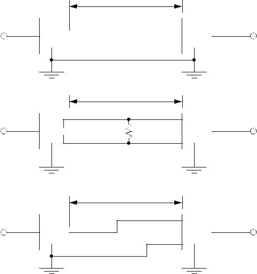
Serial communications send a single bit at a time between computers. This only requires a single communication channel, as opposed to 8 channels to send a byte. With only one channel the costs are lower, but the communication rates are slower. The communication channels are often wire based, but they may also be optical and radio. Figure 22.2 shows some of the standard electrical connections. RS-232c is the most common standard that is based on a voltage level change. At the sending computer an input will either be true or false. The ’line driver’ will convert a false value ’in’ to a ’Txd’ voltage between +3V to +15V, true will be between -3V to -15V. A cable connects the ’Txd’ and ’com’ on the sending computer to the ’Rxd’ and ’com’ inputs on the receiving computer. The receiver converts the positive and negative voltages back to logic voltage levels in the receiving computer. The cable length is limited to 50 feet to reduce the effects of electrical noise. When RS-232 is used on the factory floor, care is required to reduce the effects of electrical noise - careful grounding and shielded cables are often used.

page 120
50 ft
RS-232c
Txd |
Rxd |
In
Out
com
3000 ft
RS-422a
In
Out
3000 ft
RS-423a
In
Out
Figure 22.2 - Serial Data Standards
The RS-422a cable uses a 20 mA current loop instead of voltage levels. This makes the systems more immune to electrical noise, so the cable can be up to 3000 feet long. The RS-423a standard uses a differential voltage level across two lines, also making the system more immune to electrical noise, thus allowing longer cables. To provide serial communication in two directions these circuits must be connected in both directions.
To transmit data, the sequence of bits follows a pattern, like that shown in Figure 22.3. The

page 121
transmission starts at the left hand side. Each bit will be true or false for a fixed period of time,
determined by the transmission speed.
A typical data byte looks like the one below. The voltage/current on the line is made true or
false. The width of the bits determines the possible bits per second (bps). The value shown before
is used to transmit a single byte. Between bytes, and when the line is idle, the ’Txd’ is kept true,
this helps the receiver detect when a sender is present. A single start bit is sent by making the
’Txd’ false. In this example the next eight bits are the transmitted data, a byte with the value 17.
The data is followed by a parity bit that can be used to check the byte. In this example there are
two data bits set, and even parity is being used, so the parity bit is set. The parity bit is followed
by two stop bits to help separate this byte from the next one.
true
false
before |
start |
data |
parity |
stop |
idle |
|
|
|
|
|
Descriptions:
before - this is a period where no bit is being sent and the line is true. start - a single bit to help get the systems synchronized.
data - this could be 7 or 8 bits, but is almost always 8 now. The value shown here is a byte with the binary value 00010010 (the least significant bit is sent first).
parity - this lets us check to see if the byte was sent properly. The most common choices here are no parity bit, an even parity bit, or an odd parity bit. In this case there are two bits set in the data byte. If we are using even parity the bit would be true. If we are using odd parity the bit would be false.
stop - the stop bits allow a pause at the end of the data. One or two stop bits can be used.
idle - a period of time where the line is true before the next byte.
Figure 22.3 - A Serial Data Byte
Some of the byte settings are optional, such as the number of data bits (7 or 8), the parity bit
(none, even or odd) and the number of stop bits (1 or 2). The sending and receiving computers
must know what these settings are to properly receive and decode the data. Most computers send
page 122
the data asynchronously, meaning that the data could be sent at any time, without warning. This makes the bit settings more important.
Another method used to detect data errors is half-duplex and full-duplex transmission. In half-duplex transmission the data is only sent in one direction. But, in full-duplex transmission a copy of any byte received is sent back to the sender to verify that it was sent and received correctly. (Note: if you type and nothing shows up on a screen, or characters show up twice you may have to change the half/full duplex setting.)
The transmission speed is the maximum number of bits that can be sent per second. The units
for this is ’baud’. The baud rate includes the start, parity and stop bits. For example a 9600 baud
9600 |
= 800 |
transmission of the data in Figure 22.3 would transfer up to -----------------------------------bytes each |
|
( 1 + 8 + 1 + 2) |
|
second. Lower baud rates are 120, 300, 1.2K, 2.4K and 9.6K. Higher speeds are 19.2K, 28.8K and 33.3K. (Note: When this is set improperly you will get many transmission errors, or ’garbage’ on your screen.)
Serial lines have become one of the most common methods for transmitting data to instruments: most personal computers have two serial ports. The previous discussion of serial communications techniques also applies to devices such as modems.
6.1.1 RS-232
The RS-232c standard is based on a low/false voltage between +3 to +15V, and an high/true voltage between -3 to -15V (+/-12V is commonly used). Figure 22.4 shows some of the common connection schemes. In all methods the ’txd’ and ’rxd’ lines are crossed so that the sending ’txd’ outputs are into the listening ’rxd’ inputs when communicating between computers. When communicating with a communication device (modem), these lines are not crossed. In the ’modem’ connection the ’dsr’ and ’dtr’ lines are used to control the flow of data. In the ’computer’ the ’cts’

page 123
and ’rts’ lines are connected. These lines are all used for handshaking, to control the flow of data
from sender to receiver. The ’null-modem’ configuration simplifies the handshaking between
computers. The three wire configuration is a crude way to connect to devices, and data can be lost.
Modem
Computer
Null-Modem
Three wire
|
com |
|
|
|
|
|
|
|
|
Computer |
txd |
|
|
|
rxd |
|
|
|
|
|
|
|
|
|
|
dsr |
|
|
|
|
dtr |
|
|
|
|
|
|
|
|
|
|
|
|
|
|
|
|
|
|
|
com |
|
|
|
|
|
|
|
|
Computer |
txd |
|
|
|
|
|
|
||
rxd |
|
|
|
|
A |
|
|
|
|
cts |
|
|
|
|
|
|
|
|
|
|
rts |
|
|
|
|
|
|
|
|
com |
|
|
txd |
Modem |
|
rxd |
||
|
||
dsr |
|
|
dtr |
|
|
com |
|
|
txd |
Computer |
|
rxd |
||
B |
||
cts |
||
|
||
rts |
|
|
com |
com |
|
Computer |
txd |
txd |
Computer |
rxd |
rxd |
||
A |
dsr |
dsr |
B |
|
|
||
|
dtr |
dtr |
|
|
cts |
cts |
|
|
rts |
rts |
|
|
com |
|
|
|
|
|
com |
|
|
|
|
|
|
|
|
||
Computer |
txd |
|
|
|
|
|
txd |
Computer |
|
|
|
|
|
||||
rxd |
|
|
|
|
|
rxd |
||
A |
|
|
|
|
|
B |
||
cts |
|
|
|
|
|
cts |
||
|
|
|
|
|
|
|
||
|
rts |
|
|
|
|
|
rts |
|
|
|
|
|
|
|
|
|
|
Figure 22.4 - Common RS-232 Connection Schemes
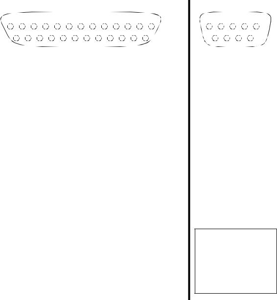
Common connectors for serial communications are shown in Figure 22.5. These connectors
are either male (with pins) or female (with holes), and often use the assigned pins shown. The
DB-9 connector is more common now, but the DB-25 connector is still in use. In any connection
the ’RXD’ and ’TXD’ pins must be used to transmit and receive data. The ’COM’ must be con-
nected to give a common voltage reference. All of the remaining pins are used for ’handshaking’.

page 124
|
|
|
|
|
|
DB-25 |
|
|
|
|
|
|
1 |
2 |
3 |
4 |
5 |
6 |
7 |
8 |
9 |
10 11 12 13 |
|||
|
14 |
15 |
16 |
17 |
18 |
19 |
20 |
21 |
22 |
23 |
24 |
25 |
Commonly used pins
1 - GND (chassis ground)
2 - TXD (transmit data)
3 - RXD (receive data)
4 - RTS (request to send)
5 - CTS (clear to send)
6 - DSR (data set ready)
7 - COM (common)
8 - DCD (Data Carrier Detect)
20 - DTR (data terminal ready) Other pins
9 - Positive Voltage
10 - Negative Voltage
11 - not used
12 - Secondary Received Line Signal Detector
13 - Secondary Clear to Send
14 - Secondary Transmitted Data
15 - Transmission Signal Element Timing (DCE)
16 - Secondary Received Data
17 - Receiver Signal Element Timing (DCE)
18 - not used
19 - Secondary Request to Send
21 - Signal Quality Detector
22 - Ring Indicator (RI)
23 - Data Signal Rate Selector (DTE/DCE)
24 - Transmit Signal Element Timing (DTE)
25 - Busy
DB-9
1 2 3 4 5
6 7 8 9
1 - DCD
2 - RXD
3 - TXD
4 - DTR
5 - COM
6 - DSR
7 - RTS
8 - CTS
9 - RI
Note: these connectors often have very small numbers printed on them to help you identify the pins.
Figure 22.5 - Typical RS-232 Pin Assignments and Names
The ’handshaking’ lines are to be used to detect the status of the sender and receiver, and to
regulate the flow of data. It would be unusual for most of these pins to be connected in any one
application. The most common pins are provided on the DB-9 connector, and are also described
below.
TXD/RXD - (transmit data, receive data) - data lines
DCD - (data carrier detect) - this indicates when a remote device is present
RI - (ring indicator) - this is used by modems to indicate when a connection is about to be