
- •1. INTEGRATED AND AUTOMATED MANUFACTURING
- •1.1 INTRODUCTION
- •1.1.1 Why Integrate?
- •1.1.2 Why Automate?
- •1.2 THE BIG PICTURE
- •1.2.2 The Architecture of Integration
- •1.2.3 General Concepts
- •1.3 PRACTICE PROBLEMS
- •2. AN INTRODUCTION TO LINUX/UNIX
- •2.1 OVERVIEW
- •2.1.1 What is it?
- •2.1.2 A (Brief) History
- •2.1.3 Hardware required and supported
- •2.1.4 Applications and uses
- •2.1.5 Advantages and Disadvantages
- •2.1.6 Getting It
- •2.1.7 Distributions
- •2.1.8 Installing
- •2.2 USING LINUX
- •2.2.1 Some Terminology
- •2.2.2 File and directories
- •2.2.3 User accounts and root
- •2.2.4 Processes
- •2.3 NETWORKING
- •2.3.1 Security
- •2.4 INTERMEDIATE CONCEPTS
- •2.4.1 Shells
- •2.4.2 X-Windows
- •2.4.3 Configuring
- •2.4.4 Desktop Tools
- •2.5 LABORATORY - A LINUX SERVER
- •2.6 TUTORIAL - INSTALLING LINUX
- •2.7 TUTORIAL - USING LINUX
- •2.8 REFERENCES
- •3. AN INTRODUCTION TO C/C++ PROGRAMMING
- •3.1 INTRODUCTION
- •3.2 PROGRAM PARTS
- •3.3 CLASSES AND OVERLOADING
- •3.4 HOW A ‘C’ COMPILER WORKS
- •3.5 STRUCTURED ‘C’ CODE
- •3.6 COMPILING C PROGRAMS IN LINUX
- •3.6.1 Makefiles
- •3.7 ARCHITECTURE OF ‘C’ PROGRAMS (TOP-DOWN)
- •3.8 CREATING TOP DOWN PROGRAMS
- •3.9 CASE STUDY - THE BEAMCAD PROGRAM
- •3.9.1 Objectives:
- •3.9.2 Problem Definition:
- •3.9.3 User Interface:
- •3.9.3.1 - Screen Layout (also see figure):
- •3.9.3.2 - Input:
- •3.9.3.3 - Output:
- •3.9.3.4 - Help:
- •3.9.3.5 - Error Checking:
- •3.9.3.6 - Miscellaneous:
- •3.9.4 Flow Program:
- •3.9.5 Expand Program:
- •3.9.6 Testing and Debugging:
- •3.9.7 Documentation
- •3.9.7.1 - Users Manual:
- •3.9.7.2 - Programmers Manual:
- •3.9.8 Listing of BeamCAD Program.
- •3.10 PRACTICE PROBLEMS
- •3.11 LABORATORY - C PROGRAMMING
- •4. NETWORK COMMUNICATION
- •4.1 INTRODUCTION
- •4.2 NETWORKS
- •4.2.1 Topology
- •4.2.2 OSI Network Model
- •4.2.3 Networking Hardware
- •4.2.4 Control Network Issues
- •4.2.5 Ethernet
- •4.2.6 SLIP and PPP
- •4.3 INTERNET
- •4.3.1 Computer Addresses
- •4.3.2 Computer Ports
- •4.3.2.1 - Mail Transfer Protocols
- •4.3.2.2 - FTP - File Transfer Protocol
- •4.3.2.3 - HTTP - Hypertext Transfer Protocol
- •4.3.3 Security
- •4.3.3.1 - Firewalls and IP Masquerading
- •4.4 FORMATS
- •4.4.1 HTML
- •4.4.2 URLs
- •4.4.3 Encryption
- •4.4.4 Clients and Servers
- •4.4.5 Java
- •4.4.6 Javascript
- •4.5 NETWORKING IN LINUX
- •4.5.1 Network Programming in Linux
- •4.6 DESIGN CASES
- •4.7 SUMMARY
- •4.8 PRACTICE PROBLEMS
- •4.9 LABORATORY - NETWORKING
- •4.9.1 Prelab
- •4.9.2 Laboratory
- •5. DATABASES
- •5.1 SQL AND RELATIONAL DATABASES
- •5.2 DATABASE ISSUES
- •5.3 LABORATORY - SQL FOR DATABASE INTEGRATION
- •5.4 LABORATORY - USING C FOR DATABASE CALLS
- •6. COMMUNICATIONS
- •6.1 SERIAL COMMUNICATIONS
- •6.2 SERIAL COMMUNICATIONS UNDER LINUX
- •6.3 PARALLEL COMMUNICATIONS
- •6.4 LABORATORY - SERIAL INTERFACING AND PROGRAMMING
- •6.5 LABORATORY - STEPPER MOTOR CONTROLLER
- •7. PROGRAMMABLE LOGIC CONTROLLERS (PLCs)
- •7.1 BASIC LADDER LOGIC
- •7.2 WHAT DOES LADDER LOGIC DO?
- •7.2.1 Connecting A PLC To A Process
- •7.2.2 PLC Operation
- •7.3 LADDER LOGIC
- •7.3.1 Relay Terminology
- •7.3.2 Ladder Logic Inputs
- •7.3.3 Ladder Logic Outputs
- •7.4 LADDER DIAGRAMS
- •7.4.1 Ladder Logic Design
- •7.4.2 A More Complicated Example of Design
- •7.5 TIMERS/COUNTERS/LATCHES
- •7.6 LATCHES
- •7.7 TIMERS
- •7.8 COUNTERS
- •7.9 DESIGN AND SAFETY
- •7.9.1 FLOW CHARTS
- •7.10 SAFETY
- •7.10.1 Grounding
- •7.10.2 Programming/Wiring
- •7.10.3 PLC Safety Rules
- •7.10.4 Troubleshooting
- •7.11 DESIGN CASES
- •7.11.1 DEADMAN SWITCH
- •7.11.2 CONVEYOR
- •7.11.3 ACCEPT/REJECT SORTING
- •7.11.4 SHEAR PRESS
- •7.12 ADDRESSING
- •7.12.1 Data Files
- •7.12.1.1 - Inputs and Outputs
- •7.12.1.2 - User Numerical Memory
- •7.12.1.3 - Timer Counter Memory
- •7.12.1.4 - PLC Status Bits (for PLC-5s)
- •7.12.1.5 - User Function Memory
- •7.13 INSTRUCTION TYPES
- •7.13.1 Program Control Structures
- •7.13.2 Branching and Looping
- •7.13.2.1 - Immediate I/O Instructions
- •7.13.2.2 - Fault Detection and Interrupts
- •7.13.3 Basic Data Handling
- •7.13.3.1 - Move Functions
- •7.14 MATH FUNCTIONS
- •7.15 LOGICAL FUNCTIONS
- •7.15.1 Comparison of Values
- •7.16 BINARY FUNCTIONS
- •7.17 ADVANCED DATA HANDLING
- •7.17.1 Multiple Data Value Functions
- •7.17.2 Block Transfer Functions
- •7.18 COMPLEX FUNCTIONS
- •7.18.1 Shift Registers
- •7.18.2 Stacks
- •7.18.3 Sequencers
- •7.19 ASCII FUNCTIONS
- •7.20 DESIGN TECHNIQUES
- •7.20.1 State Diagrams
- •7.21 DESIGN CASES
- •7.21.1 If-Then
- •7.21.2 For-Next
- •7.21.3 Conveyor
- •7.22 IMPLEMENTATION
- •7.23 PLC WIRING
- •7.23.1 SWITCHED INPUTS AND OUTPUTS
- •7.23.1.1 - Input Modules
- •7.23.1.2 - Actuators
- •7.23.1.3 - Output Modules
- •7.24 THE PLC ENVIRONMENT
- •7.24.1 Electrical Wiring Diagrams
- •7.24.2 Wiring
- •7.24.3 Shielding and Grounding
- •7.24.4 PLC Environment
- •7.24.5 SPECIAL I/O MODULES
- •7.25 PRACTICE PROBLEMS
- •7.26 REFERENCES
- •7.27 LABORATORY - SERIAL INTERFACING TO A PLC
- •8. PLCS AND NETWORKING
- •8.1 OPEN NETWORK TYPES
- •8.1.1 Devicenet
- •8.1.2 CANbus
- •8.1.3 Controlnet
- •8.1.4 Profibus
- •8.2 PROPRIETARY NETWORKS
- •8.2.0.1 - Data Highway
- •8.3 PRACTICE PROBLEMS
- •8.4 LABORATORY - DEVICENET
- •8.5 TUTORIAL - SOFTPLC AND DEVICENET
- •9. INDUSTRIAL ROBOTICS
- •9.1 INTRODUCTION
- •9.1.1 Basic Terms
- •9.1.2 Positioning Concepts
- •9.1.2.1 - Accuracy and Repeatability
- •9.1.2.2 - Control Resolution
- •9.1.2.3 - Payload
- •9.2 ROBOT TYPES
- •9.2.1 Basic Robotic Systems
- •9.2.2 Types of Robots
- •9.2.2.1 - Robotic Arms
- •9.2.2.2 - Autonomous/Mobile Robots
- •9.2.2.2.1 - Automatic Guided Vehicles (AGVs)
- •9.3 MECHANISMS
- •9.4 ACTUATORS
- •9.5 A COMMERCIAL ROBOT
- •9.5.1 Mitsubishi RV-M1 Manipulator
- •9.5.2 Movemaster Programs
- •9.5.2.0.1 - Language Examples
- •9.5.3 Command Summary
- •9.6 PRACTICE PROBLEMS
- •9.7 LABORATORY - MITSUBISHI RV-M1 ROBOT
- •9.8 TUTORIAL - MITSUBISHI RV-M1
- •10. OTHER INDUSTRIAL ROBOTS
- •10.1 SEIKO RT 3000 MANIPULATOR
- •10.1.1 DARL Programs
- •10.1.1.1 - Language Examples
- •10.1.1.2 - Commands Summary
- •10.2 IBM 7535 MANIPULATOR
- •10.2.1 AML Programs
- •10.3 ASEA IRB-1000
- •10.4 UNIMATION PUMA (360, 550, 560 SERIES)
- •10.5 PRACTICE PROBLEMS
- •10.6 LABORATORY - SEIKO RT-3000 ROBOT
- •10.7 TUTORIAL - SEIKO RT-3000 ROBOT
- •10.8 LABORATORY - ASEA IRB-1000 ROBOT
- •10.9 TUTORIAL - ASEA IRB-1000 ROBOT
- •11. ROBOT APPLICATIONS
- •11.0.1 Overview
- •11.0.2 Spray Painting and Finishing
- •11.0.3 Welding
- •11.0.4 Assembly
- •11.0.5 Belt Based Material Transfer
- •11.1 END OF ARM TOOLING (EOAT)
- •11.1.1 EOAT Design
- •11.1.2 Gripper Mechanisms
- •11.1.2.1 - Vacuum grippers
- •11.1.3 Magnetic Grippers
- •11.1.3.1 - Adhesive Grippers
- •11.1.4 Expanding Grippers
- •11.1.5 Other Types Of Grippers
- •11.2 ADVANCED TOPICS
- •11.2.1 Simulation/Off-line Programming
- •11.3 INTERFACING
- •11.4 PRACTICE PROBLEMS
- •11.5 LABORATORY - ROBOT INTERFACING
- •11.6 LABORATORY - ROBOT WORKCELL INTEGRATION
- •12. SPATIAL KINEMATICS
- •12.1 BASICS
- •12.1.1 Degrees of Freedom
- •12.2 HOMOGENEOUS MATRICES
- •12.2.1 Denavit-Hartenberg Transformation (D-H)
- •12.2.2 Orientation
- •12.2.3 Inverse Kinematics
- •12.2.4 The Jacobian
- •12.3 SPATIAL DYNAMICS
- •12.3.1 Moments of Inertia About Arbitrary Axes
- •12.3.2 Euler’s Equations of Motion
- •12.3.3 Impulses and Momentum
- •12.3.3.1 - Linear Momentum
- •12.3.3.2 - Angular Momentum
- •12.4 DYNAMICS FOR KINEMATICS CHAINS
- •12.4.1 Euler-Lagrange
- •12.4.2 Newton-Euler
- •12.5 REFERENCES
- •12.6 PRACTICE PROBLEMS
- •13. MOTION CONTROL
- •13.1 KINEMATICS
- •13.1.1 Basic Terms
- •13.1.2 Kinematics
- •13.1.2.1 - Geometry Methods for Forward Kinematics
- •13.1.2.2 - Geometry Methods for Inverse Kinematics
- •13.1.3 Modeling the Robot
- •13.2 PATH PLANNING
- •13.2.1 Slew Motion
- •13.2.1.1 - Joint Interpolated Motion
- •13.2.1.2 - Straight-line motion
- •13.2.2 Computer Control of Robot Paths (Incremental Interpolation)
- •13.3 PRACTICE PROBLEMS
- •13.4 LABORATORY - AXIS AND MOTION CONTROL
- •14. CNC MACHINES
- •14.1 MACHINE AXES
- •14.2 NUMERICAL CONTROL (NC)
- •14.2.1 NC Tapes
- •14.2.2 Computer Numerical Control (CNC)
- •14.2.3 Direct/Distributed Numerical Control (DNC)
- •14.3 EXAMPLES OF EQUIPMENT
- •14.3.1 EMCO PC Turn 50
- •14.3.2 Light Machines Corp. proLIGHT Mill
- •14.4 PRACTICE PROBLEMS
- •14.5 TUTORIAL - EMCO MAIER PCTURN 50 LATHE (OLD)
- •14.6.1 LABORATORY - CNC MACHINING
- •15. CNC PROGRAMMING
- •15.1 G-CODES
- •15.3 PROPRIETARY NC CODES
- •15.4 GRAPHICAL PART PROGRAMMING
- •15.5 NC CUTTER PATHS
- •15.6 NC CONTROLLERS
- •15.7 PRACTICE PROBLEMS
- •15.8 LABORATORY - CNC INTEGRATION
- •16. DATA AQUISITION
- •16.1 INTRODUCTION
- •16.2 ANALOG INPUTS
- •16.3 ANALOG OUTPUTS
- •16.4 REAL-TIME PROCESSING
- •16.5 DISCRETE IO
- •16.6 COUNTERS AND TIMERS
- •16.7 ACCESSING DAQ CARDS FROM LINUX
- •16.8 SUMMARY
- •16.9 PRACTICE PROBLEMS
- •16.10 LABORATORY - INTERFACING TO A DAQ CARD
- •17. VISIONS SYSTEMS
- •17.1 OVERVIEW
- •17.2 APPLICATIONS
- •17.3 LIGHTING AND SCENE
- •17.4 CAMERAS
- •17.5 FRAME GRABBER
- •17.6 IMAGE PREPROCESSING
- •17.7 FILTERING
- •17.7.1 Thresholding
- •17.8 EDGE DETECTION
- •17.9 SEGMENTATION
- •17.9.1 Segment Mass Properties
- •17.10 RECOGNITION
- •17.10.1 Form Fitting
- •17.10.2 Decision Trees
- •17.11 PRACTICE PROBLEMS
- •17.12 TUTORIAL - LABVIEW BASED IMAQ VISION
- •17.13 LABORATORY - VISION SYSTEMS FOR INSPECTION
- •18. INTEGRATION ISSUES
- •18.1 CORPORATE STRUCTURES
- •18.2 CORPORATE COMMUNICATIONS
- •18.3 COMPUTER CONTROLLED BATCH PROCESSES
- •18.4 PRACTICE PROBLEMS
- •18.5 LABORATORY - WORKCELL INTEGRATION
- •19. MATERIAL HANDLING
- •19.1 INTRODUCTION
- •19.2 VIBRATORY FEEDERS
- •19.3 PRACTICE QUESTIONS
- •19.4 LABORATORY - MATERIAL HANDLING SYSTEM
- •19.4.1 System Assembly and Simple Controls
- •19.5 AN EXAMPLE OF AN FMS CELL
- •19.5.1 Overview
- •19.5.2 Workcell Specifications
- •19.5.3 Operation of The Cell
- •19.6 THE NEED FOR CONCURRENT PROCESSING
- •19.7 PRACTICE PROBLEMS
- •20. PETRI NETS
- •20.1 INTRODUCTION
- •20.2 A BRIEF OUTLINE OF PETRI NET THEORY
- •20.3 MORE REVIEW
- •20.4 USING THE SUBROUTINES
- •20.4.1 Basic Petri Net Simulation
- •20.4.2 Transitions With Inhibiting Inputs
- •20.4.3 An Exclusive OR Transition:
- •20.4.4 Colored Tokens
- •20.4.5 RELATIONAL NETS
- •20.5 C++ SOFTWARE
- •20.6 IMPLEMENTATION FOR A PLC
- •20.7 PRACTICE PROBLEMS
- •20.8 REFERENCES
- •21. PRODUCTION PLANNING AND CONTROL
- •21.1 OVERVIEW
- •21.2 SCHEDULING
- •21.2.1 Material Requirements Planning (MRP)
- •21.2.2 Capacity Planning
- •21.3 SHOP FLOOR CONTROL
- •21.3.1 Shop Floor Scheduling - Priority Scheduling
- •21.3.2 Shop Floor Monitoring
- •22. SIMULATION
- •22.1 MODEL BUILDING
- •22.2 ANALYSIS
- •22.3 DESIGN OF EXPERIMENTS
- •22.4 RUNNING THE SIMULATION
- •22.5 DECISION MAKING STRATEGY
- •23. PLANNING AND ANALYSIS
- •23.1 FACTORS TO CONSIDER
- •23.2 PROJECT COST ACCOUNTING
- •24. REFERENCES
- •25. APPENDIX A - PROJECTS
- •25.1 TOPIC SELECTION
- •25.1.1 Previous Project Topics
- •25.2 CURRENT PROJECT DESCRIPTIONS
- •26. APPENDIX B - COMMON REFERENCES
- •26.1 JIC ELECTRICAL SYMBOLS
- •26.2 NEMA ENCLOSURES
page 73
resuming transmission if it is interrupted or corrupted. The ’Session’ layer will often make long term connections to the remote machine. The ’Presentation’ layer acts as an application interface so that syntax, formats and codes are consistent between the two networked machines. For example this might convert ’\’ to ’/’ in HTML files. This layer also provides subroutines that the user may call to access network functions, and perform functions such as encryption and compression. The ’Application’ layer is where the user program resides. On a computer this might be a web browser, or a ladder logic program on a PLC.
Most products can be described with only a couple of layers. Some networking products may omit layers in the model. Consider the networks shown in Figure 22.15.
4.2.3 Networking Hardware
The following is a description of most of the hardware that will be needed in the design of networks.
•Computer (or network enabled equipment)
•Network Interface Hardware - The network interface may already be built into the computer/PLC/sensor/etc. These may cost $15 to over $1000.
•The Media - The physical network connection between network nodes.
10baseT (twisted pair) is the most popular. It is a pair of twisted copper wires terminated with an RJ-45 connector.
10base2 (thin wire) is thin shielded coaxial cable with BNC connectors 10baseF (fiber optic) is costly, but signal transmission and noise properties are
very good.
•Repeaters (Physical Layer) - These accept signals and retransmit them so that longer networks can be built.
•Hub/Concentrator - A central connection point that network wires will be connected to. It will pass network packets to local computers, or to remote networks if they are available.
•Router (Network Layer) - Will isolate different networks, but redirect traffic to other LANs.
•Bridges (Data link layer) - These are intelligent devices that can convert data on one type of network, to data on another type of network. These can also be used to isolate two networks.

page 74
• Gateway (Application Layer) - A Gateway is a full computer that will direct traffic to different networks, and possibly screen packets. These are often used to create firewalls for security.
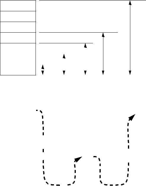
Figure 22.15 shows the basic OSI model equivalents for some of the networking hardware
described before.
7 - application
6 - presentation |
gateway |
5 - session
4 - transport
3 |
- network |
|
|
|
|
|
|
|
|
switch |
|
|
|
|
|
|
|
|
|||
|
|
|
|
|
|
|
|
|
|
|
2 |
- data link |
|
|
|
|
|
bridge |
|
router |
|
|
|
|
|
|
||||||
|
|
|
|
|
|
|
|
|
||
1 |
- physical |
|
repeater |
|||||||
|
|
|
|
|
|
|||||
|
|
|||||||||
|
|
|
|
|||||||
|
|
|
|
|
|
|
|
|
|
|
Figure 22.15 - Network Devices and the OSI Model
Layer |
Computer #1 |
|
|
|
|
|
|
|
|
|
|
|
|
|
|
|
|
Computer #2 |
|
|
|
|
|
|
|
|
|
|
|
|
|
|
|
|
|
|
|
|
|
7 |
Application |
|
|
|
|
|
|
|
|
|
|
|
|
|
|
|
|
Application |
|
|
|
|
|
|
|
|
|
|
|
|
|
|
|
|
|
|
|
|
|
6 |
Presentation |
|
|
|
|
|
|
|
|
|
|
|
|
|
|
|
|
Presentation |
|
|
|
|
|
|
|
|
|
|
|
|
|
|
|
|
|
|
|
|
|
5 |
Session |
|
|
|
|
|
|
|
|
|
|
|
|
|
|
|
|
Session |
|
|
|
|
|
|
|
|
|
|
|
|
Router |
|
|
||||||
|
|
|
|
|
|
|
|
|
|
|
|
|
|||||||
4 |
Transport |
Transport |
|
||||||||||||||||
|
|
|
|
|
|
|
|
|
|
||||||||||
|
|
|
|
|
|
|
|
|
|
|
|
|
|
|
|
|
|||
|
|
|
|
|
|
|
|
|
|
|
|
|
|
|
|
|
|||
|
|
|
|
|
|
|
|
|
|
|
|
|
|
|
|
|
|
|
|
3 |
Network |
|
|
|
|
|
|
|
|
|
Network |
|
Network |
|
|||||
|
|
|
|
|
|
|
|
|
|
|
|||||||||
|
|
|
|
|
|
|
|
|
|
|
|||||||||
|
|
|
|
|
|
|
|
|
|
|
|
|
|
|
|
|
|
|
|
|
|
|
|
|
|
|
|
|
|
|
|
|
|
|
|
|
|
|
|
2 |
Data Link |
|
|
|
|
|
|
|
|
|
Data Link |
|
|
|
Data Link |
|
|||
|
|
|
|
|
|
|
|
|
|
|
|
|
|||||||
|
|
|
|
|
|
|
|
|
|
|
|
|
|
|
|
|
|
|
|
1 |
Physical |
|
|
|
|
|
|
|
|
|
Physical |
|
Physical |
|
|||||
|
|
|
|
|
|
|
|
|
|
|
|
|
|
|
|
|
|
|
|
|
|
|
|
|
|
|
|
|
|
|
|
|
|
|
|
|
|
|
|
|
|
|
|
|
|
|
|
Interconnecting Medium |
|
|
|||||||||
|
|
|
|
|
|
|
|
|
|
|
|
|
|
|
|
|
|
|
|
Figure 22.15X - The OSI Network Model with a Router
page 75
4.2.4 Control Network Issues
A wide variety of networks are commercially available, and each has particular strengths and weaknesses. The differences arise from their basic designs. One simple issue is the use of the network to deliver power to the nodes. Some control networks will also supply enough power to drive some sensors and simple devices. This can eliminate separate power supplies, but it can reduce the data transmission rates on the network. The use of network taps or tees to connect to the network cable is also important. Some taps or tees are simple ’passive’ electrical connections, but others involve sophisticated ’active’ tees that are more costly, but allow longer networks.
The transmission type determines the communication speed and noise immunity. The simplest transmission method is baseband, where voltages are switched off and on to signal bit states. This method is subject to noise, and must operate at lower speeds. RS-232 is an example of baseband transmission. Carrierband transmission uses FSK (Frequency Shift Keying) that will switch a signal between two frequencies to indicate a true or false bit. This technique is very similar to FM (Frequency Modulation) radio where the frequency of the audio wave is transmitted by changing the frequency of a carrier frequency about 100MHz. This method allows higher transmission speeds, with reduced noise effects. Broadband networks transmit data over more than one channel by using multiple carrier frequencies on the same wire. This is similar to sending many cable television channels over the same wire. These networks can achieve very large transmission speeds, and can also be used to guarantee real time network access.
The bus network topology only uses a single transmission wire for all nodes. If all of the nodes decide to send messages simultaneously, the messages would be corrupted (a collision occurs). There are a variety of methods for dealing with network collisions, and arbitration.
CSMA/CD (Collision Sense Multiple Access/Collision Detection) - if two nodes start talking and detect a collision then they will stop, wait a random time, and then start again.
CSMA/BA (Collision Sense Multiple Access/Bitwise Arbitration) - if two nodes start
page 76
talking at the same time the will stop and use their node addresses to determine which one goes first.
Master-Slave - one device one the network is the master and is the only one that may start communication. slave devices will only respond to requests from the master.
Token Passing - A token, or permission to talk, is passed sequentially around a network so that only one station may talk at a time.
The token passing method is deterministic, but it may require that a node with an urgent message wait to receive the token. The master-slave method will put a single machine in charge of sending and receiving. This can be restrictive if multiple controllers are to exist on the same network. The CSMA/CD and CSMA/BA methods will both allow nodes to talk when needed. But, as the number of collisions increase the network performance degrades quickly.
4.2.5 Ethernet
Ethernet has become the predominate networking format. Version I was released in 1980 by a consortium of companies. In the 1980s various versions of ethernet frames were released. These include Version II and Novell Networking (IEEE 802.3). Most modern ethernet cards will support different types of frames.
The ethernet frame is shown in Figure 20.21. The first six bytes are the destination address for the message. If all of the bits in the bytes are set then any computer that receives the message will read it. The first three bytes of the address are specific to the card manufacturer, and the remaining bytes specify the remote address. The address is common for all versions of ethernet. The source address specifies the message sender. The first three bytes are specific to the card manufacturer. The remaining bytes include the source address. This is also identical in all versions of ethernet. The ’ethernet type’ identifies the frame as aVersion II ethernet packet if the value is greater than 05DChex. The other ethernet types use these to bytes to indicate the datalength. The ’data’ can be between 46 to 1500 bytes in length. The frame concludes with a ’checksum’ that will be used to verify that the data has been transmitted correctly. When the end of the transmission is detected, the last four bytes are then used to verify that the frame was received