


page 50
memory. The computer remembers where the location of that variable is, this memory of location is called a pointer. This pointer is always hidden from the programmer, and uses it only in the background. In ‘C’, the pointer to a variable may be used. We may use some of the operations of ‘C’ to get the variable that the pointer, points to. This allows us to deal with variables in a very powerful way.
#include “stdio.h”
main() {
int i;
char *string; /* character pointer */ gets(string); /* Input string from keyboard */ for(i = 0; string[i] != 0; i++){
printf(“ pos %d, char %c, ASCII %d \n”, i, string[i], string[i]);
}
}
INPUT:
HUGH<return>
OUTPUT:
pos 0, char H, ASCII 72 pos 1, char U, ASCII 85 pos 2, char G, ASCII 71 pos 3, char H, ASCII 72
Figure 3.10 - A Sample Program to Get a String
3.3 CLASSES AND OVERLOADING
Classes are the core concept behind object oriented programing. They basically allow data and functions to be grouped together into a complex data type. The example code below shows a class definition, and a program that uses it.
page 51
class bill { public:
int |
value; |
void |
result(); |
}
bill::result(){
printf("The result is %d \n", value);
};
main(){
bill A; bill B;
A.value = 3;
B.value = 5;
A.result();
B.result();
}
PROGRAM OUTPUT:
The result is 3
The result is 5
Figure 3.11 - A Simple Class Definition
The class is defined to have a public integer called’value’ and a public function called ’result’. The function ’result’ is defined separately outside of the class definition. In the ’main’ program the class has two instances ’A’ and ’B’. The ’value’ values in the classes are set, and then the result function is then called.
A more sophisticated example of a class definition follows. The program shown does exactly the same as the last program, but with some useful differences. This class now includes a constructor function ’bill’. This function is automatically called when a new instance of ’bill’ is created. In the main program the instances are not created initially, but pointers ’*A’ and ’*B’ are created. These are then assigned instances with the calls to ’new bill()’. At this point the constructor functions are called. Finally, when the instances are used, because they are pointers, the ’->’ are used instead of ’.’.
page 52
class bill { public:
bill(int);
int value; void result();
}
bill::bill(int new_value){ value = new_value;
}
bill::result(){
printf("The result is %d \n", value);
};
main(){
bill *A; bill *B;
A = new bill(3);
B = new bill(5);
A->result();
B->result();
}
PROGRAM OUTPUT:
The result is 3
The result is 5
Figure 3.12 - Another Class Example
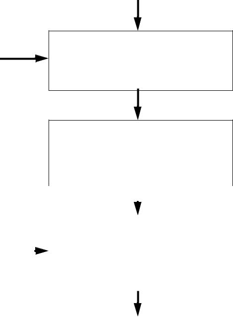
3.4 HOW A ‘C’ COMPILER WORKS
A ‘C’ compiler has three basic components: Preprocessor, First and Second Pass Compiler,
and Linker.
page 53
#include files (like “stdio.h”)
Source code “filename.c”
The Preprocessor
Will remove comments, replace strings which have a defined value, include programs, and remove unneeded characters.
ASCII Text Code
The First and Second Pass
The compiler will parse the program and check the syntax. TheSecond Pass produces some simple machine language, which performs the basic functions of the program.
|
|
|
|
|
|
|
|
|
|
|
|
Object Code (*.o) |
|
|
|
|
|
|
|
|
|
|
|
The Linker |
|
||
|
|
|
The compiler will combine the basic machine language |
|
||
|
|
|
from the first pass and combine it with the pieces of |
|
||
|
|
|
machine language in the compiler libraries. An opti- |
|
||
|
|
|
|
|||
Library files |
|
|||||
mization operation may be used to reduce execution |
|
|||||
(*.so) |
time. |
|
||||
|
|
|
|
|
|
|
Executable Code
(*.exe)
Figure 3.13 - How Programs Are Compiled