page 479

17. VISIONS SYSTEMS

• Vision systems are suited to applications where simpler sensors do not work.

17.1 OVERVIEW

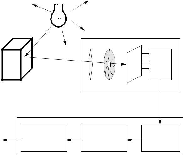
• Typical components in a modern vision system.

page 480

Lighting

Scene

Camera

lens iris

CCD control electronics

17.2 APPLICATIONS

• An example of a common vision system application is given below. The basic operation involves a belt that carries pop (soda) bottles along. As these bottles pass an optical sensor, it triggers a vision system to do a comparison. The system compares the captured image to stored images of acceptable bottles (with no foreign objects or cracks). If the bottle differs from the acceptable images beyond an acceptable margin, then a piston is fired to eject the bottle. (Note:

page 482

•Boundary edges are used when trying to determine object identity/location/orientation. This requires a high contrast between object and background so that the edges are obvious.

•Surface texture/pattern can be used to verify various features, for example - are numbered buttons in a telephone keypad in the correct positions? Some visually significant features must be present.

•Lighting,

-multiple light sources can reduce shadows (structured lighting).

-back lighting with luminescent screens can provide good contrast.

-lighting positions can reduce specular reflections (light diffusers help).

-artificial light sources provide repeatability required by vision systems that is not possible without natural light sources.

17.4 CAMERAS

•Cameras use available light from a scene.

•The light passes through a lens that focuses the beams on a plane inside the camera. The focal distance of the lens can be moved toward/away from the plane in the camera as the scene is moved towards/away.

•An iris may also be used to mechanically reduce the amount of light when the intensity is too high.

•The plane inside the camera that the light is focussed on can read the light a number of ways, but basically the camera scans the plane in a raster pattern.

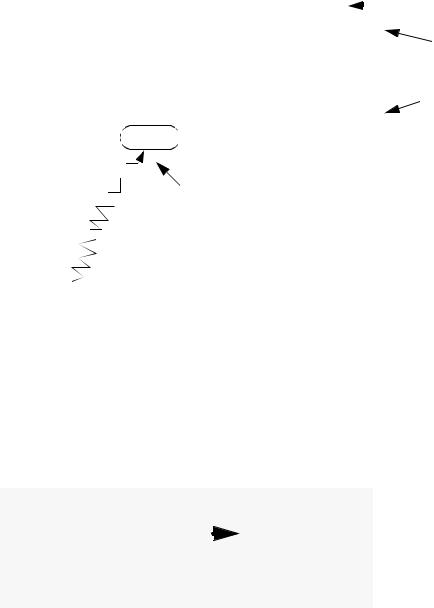
•An electron gun video camera is shown below. - The tube works like a standard CRT, the electron beam is generated by heating a cathode to eject electrons, and applying a potential between the anode and cathode to accelerate the electrons off of the cathode. The focussing/ deflecting coils can focus the beam using a similar potential change, or deflect the beam using a

page 483

differential potential. The significant effect occurs at the front of the tube. The beam is scanned over the front. Where the beam is incident it will cause electrons to jump between the plates proportional to the light intensity at that point. The scanning occurs in a raster pattern, scanning many lines left to right, top to bottom. The pattern is repeated some number of times a second - the typical refresh rate is on the order of 30Hz

electron accelerator

photon

heated cathode

scanning electron beam

anode

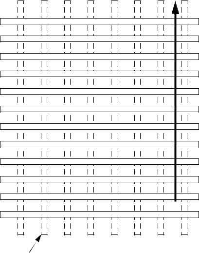
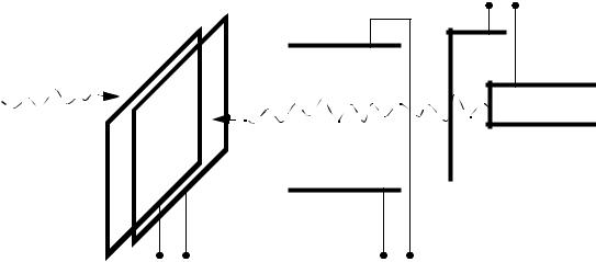
• Charge Coupled Device (CCD) - This is a newer solid state video capture technique. An array of cells are laid out on a semiconductor chip. A grid like array of conductors and insulators is used to move a collection of charge through the device. As the charge moves, it sweeps across the picture. As photons strike the semiconductor they knock an electron out of orbit, creating a negative and positive charge. The positive charges are then accumulated to determine light intensity. The mechanism for a single scan line is seen below.