
- •1. INTEGRATED AND AUTOMATED MANUFACTURING
- •1.1 INTRODUCTION
- •1.1.1 Why Integrate?
- •1.1.2 Why Automate?
- •1.2 THE BIG PICTURE
- •1.2.2 The Architecture of Integration
- •1.2.3 General Concepts
- •1.3 PRACTICE PROBLEMS
- •2. AN INTRODUCTION TO LINUX/UNIX
- •2.1 OVERVIEW
- •2.1.1 What is it?
- •2.1.2 A (Brief) History
- •2.1.3 Hardware required and supported
- •2.1.4 Applications and uses
- •2.1.5 Advantages and Disadvantages
- •2.1.6 Getting It
- •2.1.7 Distributions
- •2.1.8 Installing
- •2.2 USING LINUX
- •2.2.1 Some Terminology
- •2.2.2 File and directories
- •2.2.3 User accounts and root
- •2.2.4 Processes
- •2.3 NETWORKING
- •2.3.1 Security
- •2.4 INTERMEDIATE CONCEPTS
- •2.4.1 Shells
- •2.4.2 X-Windows
- •2.4.3 Configuring
- •2.4.4 Desktop Tools
- •2.5 LABORATORY - A LINUX SERVER
- •2.6 TUTORIAL - INSTALLING LINUX
- •2.7 TUTORIAL - USING LINUX
- •2.8 REFERENCES
- •3. AN INTRODUCTION TO C/C++ PROGRAMMING
- •3.1 INTRODUCTION
- •3.2 PROGRAM PARTS
- •3.3 CLASSES AND OVERLOADING
- •3.4 HOW A ‘C’ COMPILER WORKS
- •3.5 STRUCTURED ‘C’ CODE
- •3.6 COMPILING C PROGRAMS IN LINUX
- •3.6.1 Makefiles
- •3.7 ARCHITECTURE OF ‘C’ PROGRAMS (TOP-DOWN)
- •3.8 CREATING TOP DOWN PROGRAMS
- •3.9 CASE STUDY - THE BEAMCAD PROGRAM
- •3.9.1 Objectives:
- •3.9.2 Problem Definition:
- •3.9.3 User Interface:
- •3.9.3.1 - Screen Layout (also see figure):
- •3.9.3.2 - Input:
- •3.9.3.3 - Output:
- •3.9.3.4 - Help:
- •3.9.3.5 - Error Checking:
- •3.9.3.6 - Miscellaneous:
- •3.9.4 Flow Program:
- •3.9.5 Expand Program:
- •3.9.6 Testing and Debugging:
- •3.9.7 Documentation
- •3.9.7.1 - Users Manual:
- •3.9.7.2 - Programmers Manual:
- •3.9.8 Listing of BeamCAD Program.
- •3.10 PRACTICE PROBLEMS
- •3.11 LABORATORY - C PROGRAMMING
- •4. NETWORK COMMUNICATION
- •4.1 INTRODUCTION
- •4.2 NETWORKS
- •4.2.1 Topology
- •4.2.2 OSI Network Model
- •4.2.3 Networking Hardware
- •4.2.4 Control Network Issues
- •4.2.5 Ethernet
- •4.2.6 SLIP and PPP
- •4.3 INTERNET
- •4.3.1 Computer Addresses
- •4.3.2 Computer Ports
- •4.3.2.1 - Mail Transfer Protocols
- •4.3.2.2 - FTP - File Transfer Protocol
- •4.3.2.3 - HTTP - Hypertext Transfer Protocol
- •4.3.3 Security
- •4.3.3.1 - Firewalls and IP Masquerading
- •4.4 FORMATS
- •4.4.1 HTML
- •4.4.2 URLs
- •4.4.3 Encryption
- •4.4.4 Clients and Servers
- •4.4.5 Java
- •4.4.6 Javascript
- •4.5 NETWORKING IN LINUX
- •4.5.1 Network Programming in Linux
- •4.6 DESIGN CASES
- •4.7 SUMMARY
- •4.8 PRACTICE PROBLEMS
- •4.9 LABORATORY - NETWORKING
- •4.9.1 Prelab
- •4.9.2 Laboratory
- •5. DATABASES
- •5.1 SQL AND RELATIONAL DATABASES
- •5.2 DATABASE ISSUES
- •5.3 LABORATORY - SQL FOR DATABASE INTEGRATION
- •5.4 LABORATORY - USING C FOR DATABASE CALLS
- •6. COMMUNICATIONS
- •6.1 SERIAL COMMUNICATIONS
- •6.2 SERIAL COMMUNICATIONS UNDER LINUX
- •6.3 PARALLEL COMMUNICATIONS
- •6.4 LABORATORY - SERIAL INTERFACING AND PROGRAMMING
- •6.5 LABORATORY - STEPPER MOTOR CONTROLLER
- •7. PROGRAMMABLE LOGIC CONTROLLERS (PLCs)
- •7.1 BASIC LADDER LOGIC
- •7.2 WHAT DOES LADDER LOGIC DO?
- •7.2.1 Connecting A PLC To A Process
- •7.2.2 PLC Operation
- •7.3 LADDER LOGIC
- •7.3.1 Relay Terminology
- •7.3.2 Ladder Logic Inputs
- •7.3.3 Ladder Logic Outputs
- •7.4 LADDER DIAGRAMS
- •7.4.1 Ladder Logic Design
- •7.4.2 A More Complicated Example of Design
- •7.5 TIMERS/COUNTERS/LATCHES
- •7.6 LATCHES
- •7.7 TIMERS
- •7.8 COUNTERS
- •7.9 DESIGN AND SAFETY
- •7.9.1 FLOW CHARTS
- •7.10 SAFETY
- •7.10.1 Grounding
- •7.10.2 Programming/Wiring
- •7.10.3 PLC Safety Rules
- •7.10.4 Troubleshooting
- •7.11 DESIGN CASES
- •7.11.1 DEADMAN SWITCH
- •7.11.2 CONVEYOR
- •7.11.3 ACCEPT/REJECT SORTING
- •7.11.4 SHEAR PRESS
- •7.12 ADDRESSING
- •7.12.1 Data Files
- •7.12.1.1 - Inputs and Outputs
- •7.12.1.2 - User Numerical Memory
- •7.12.1.3 - Timer Counter Memory
- •7.12.1.4 - PLC Status Bits (for PLC-5s)
- •7.12.1.5 - User Function Memory
- •7.13 INSTRUCTION TYPES
- •7.13.1 Program Control Structures
- •7.13.2 Branching and Looping
- •7.13.2.1 - Immediate I/O Instructions
- •7.13.2.2 - Fault Detection and Interrupts
- •7.13.3 Basic Data Handling
- •7.13.3.1 - Move Functions
- •7.14 MATH FUNCTIONS
- •7.15 LOGICAL FUNCTIONS
- •7.15.1 Comparison of Values
- •7.16 BINARY FUNCTIONS
- •7.17 ADVANCED DATA HANDLING
- •7.17.1 Multiple Data Value Functions
- •7.17.2 Block Transfer Functions
- •7.18 COMPLEX FUNCTIONS
- •7.18.1 Shift Registers
- •7.18.2 Stacks
- •7.18.3 Sequencers
- •7.19 ASCII FUNCTIONS
- •7.20 DESIGN TECHNIQUES
- •7.20.1 State Diagrams
- •7.21 DESIGN CASES
- •7.21.1 If-Then
- •7.21.2 For-Next
- •7.21.3 Conveyor
- •7.22 IMPLEMENTATION
- •7.23 PLC WIRING
- •7.23.1 SWITCHED INPUTS AND OUTPUTS
- •7.23.1.1 - Input Modules
- •7.23.1.2 - Actuators
- •7.23.1.3 - Output Modules
- •7.24 THE PLC ENVIRONMENT
- •7.24.1 Electrical Wiring Diagrams
- •7.24.2 Wiring
- •7.24.3 Shielding and Grounding
- •7.24.4 PLC Environment
- •7.24.5 SPECIAL I/O MODULES
- •7.25 PRACTICE PROBLEMS
- •7.26 REFERENCES
- •7.27 LABORATORY - SERIAL INTERFACING TO A PLC
- •8. PLCS AND NETWORKING
- •8.1 OPEN NETWORK TYPES
- •8.1.1 Devicenet
- •8.1.2 CANbus
- •8.1.3 Controlnet
- •8.1.4 Profibus
- •8.2 PROPRIETARY NETWORKS
- •8.2.0.1 - Data Highway
- •8.3 PRACTICE PROBLEMS
- •8.4 LABORATORY - DEVICENET
- •8.5 TUTORIAL - SOFTPLC AND DEVICENET
- •9. INDUSTRIAL ROBOTICS
- •9.1 INTRODUCTION
- •9.1.1 Basic Terms
- •9.1.2 Positioning Concepts
- •9.1.2.1 - Accuracy and Repeatability
- •9.1.2.2 - Control Resolution
- •9.1.2.3 - Payload
- •9.2 ROBOT TYPES
- •9.2.1 Basic Robotic Systems
- •9.2.2 Types of Robots
- •9.2.2.1 - Robotic Arms
- •9.2.2.2 - Autonomous/Mobile Robots
- •9.2.2.2.1 - Automatic Guided Vehicles (AGVs)
- •9.3 MECHANISMS
- •9.4 ACTUATORS
- •9.5 A COMMERCIAL ROBOT
- •9.5.1 Mitsubishi RV-M1 Manipulator
- •9.5.2 Movemaster Programs
- •9.5.2.0.1 - Language Examples
- •9.5.3 Command Summary
- •9.6 PRACTICE PROBLEMS
- •9.7 LABORATORY - MITSUBISHI RV-M1 ROBOT
- •9.8 TUTORIAL - MITSUBISHI RV-M1
- •10. OTHER INDUSTRIAL ROBOTS
- •10.1 SEIKO RT 3000 MANIPULATOR
- •10.1.1 DARL Programs
- •10.1.1.1 - Language Examples
- •10.1.1.2 - Commands Summary
- •10.2 IBM 7535 MANIPULATOR
- •10.2.1 AML Programs
- •10.3 ASEA IRB-1000
- •10.4 UNIMATION PUMA (360, 550, 560 SERIES)
- •10.5 PRACTICE PROBLEMS
- •10.6 LABORATORY - SEIKO RT-3000 ROBOT
- •10.7 TUTORIAL - SEIKO RT-3000 ROBOT
- •10.8 LABORATORY - ASEA IRB-1000 ROBOT
- •10.9 TUTORIAL - ASEA IRB-1000 ROBOT
- •11. ROBOT APPLICATIONS
- •11.0.1 Overview
- •11.0.2 Spray Painting and Finishing
- •11.0.3 Welding
- •11.0.4 Assembly
- •11.0.5 Belt Based Material Transfer
- •11.1 END OF ARM TOOLING (EOAT)
- •11.1.1 EOAT Design
- •11.1.2 Gripper Mechanisms
- •11.1.2.1 - Vacuum grippers
- •11.1.3 Magnetic Grippers
- •11.1.3.1 - Adhesive Grippers
- •11.1.4 Expanding Grippers
- •11.1.5 Other Types Of Grippers
- •11.2 ADVANCED TOPICS
- •11.2.1 Simulation/Off-line Programming
- •11.3 INTERFACING
- •11.4 PRACTICE PROBLEMS
- •11.5 LABORATORY - ROBOT INTERFACING
- •11.6 LABORATORY - ROBOT WORKCELL INTEGRATION
- •12. SPATIAL KINEMATICS
- •12.1 BASICS
- •12.1.1 Degrees of Freedom
- •12.2 HOMOGENEOUS MATRICES
- •12.2.1 Denavit-Hartenberg Transformation (D-H)
- •12.2.2 Orientation
- •12.2.3 Inverse Kinematics
- •12.2.4 The Jacobian
- •12.3 SPATIAL DYNAMICS
- •12.3.1 Moments of Inertia About Arbitrary Axes
- •12.3.2 Euler’s Equations of Motion
- •12.3.3 Impulses and Momentum
- •12.3.3.1 - Linear Momentum
- •12.3.3.2 - Angular Momentum
- •12.4 DYNAMICS FOR KINEMATICS CHAINS
- •12.4.1 Euler-Lagrange
- •12.4.2 Newton-Euler
- •12.5 REFERENCES
- •12.6 PRACTICE PROBLEMS
- •13. MOTION CONTROL
- •13.1 KINEMATICS
- •13.1.1 Basic Terms
- •13.1.2 Kinematics
- •13.1.2.1 - Geometry Methods for Forward Kinematics
- •13.1.2.2 - Geometry Methods for Inverse Kinematics
- •13.1.3 Modeling the Robot
- •13.2 PATH PLANNING
- •13.2.1 Slew Motion
- •13.2.1.1 - Joint Interpolated Motion
- •13.2.1.2 - Straight-line motion
- •13.2.2 Computer Control of Robot Paths (Incremental Interpolation)
- •13.3 PRACTICE PROBLEMS
- •13.4 LABORATORY - AXIS AND MOTION CONTROL
- •14. CNC MACHINES
- •14.1 MACHINE AXES
- •14.2 NUMERICAL CONTROL (NC)
- •14.2.1 NC Tapes
- •14.2.2 Computer Numerical Control (CNC)
- •14.2.3 Direct/Distributed Numerical Control (DNC)
- •14.3 EXAMPLES OF EQUIPMENT
- •14.3.1 EMCO PC Turn 50
- •14.3.2 Light Machines Corp. proLIGHT Mill
- •14.4 PRACTICE PROBLEMS
- •14.5 TUTORIAL - EMCO MAIER PCTURN 50 LATHE (OLD)
- •14.6.1 LABORATORY - CNC MACHINING
- •15. CNC PROGRAMMING
- •15.1 G-CODES
- •15.3 PROPRIETARY NC CODES
- •15.4 GRAPHICAL PART PROGRAMMING
- •15.5 NC CUTTER PATHS
- •15.6 NC CONTROLLERS
- •15.7 PRACTICE PROBLEMS
- •15.8 LABORATORY - CNC INTEGRATION
- •16. DATA AQUISITION
- •16.1 INTRODUCTION
- •16.2 ANALOG INPUTS
- •16.3 ANALOG OUTPUTS
- •16.4 REAL-TIME PROCESSING
- •16.5 DISCRETE IO
- •16.6 COUNTERS AND TIMERS
- •16.7 ACCESSING DAQ CARDS FROM LINUX
- •16.8 SUMMARY
- •16.9 PRACTICE PROBLEMS
- •16.10 LABORATORY - INTERFACING TO A DAQ CARD
- •17. VISIONS SYSTEMS
- •17.1 OVERVIEW
- •17.2 APPLICATIONS
- •17.3 LIGHTING AND SCENE
- •17.4 CAMERAS
- •17.5 FRAME GRABBER
- •17.6 IMAGE PREPROCESSING
- •17.7 FILTERING
- •17.7.1 Thresholding
- •17.8 EDGE DETECTION
- •17.9 SEGMENTATION
- •17.9.1 Segment Mass Properties
- •17.10 RECOGNITION
- •17.10.1 Form Fitting
- •17.10.2 Decision Trees
- •17.11 PRACTICE PROBLEMS
- •17.12 TUTORIAL - LABVIEW BASED IMAQ VISION
- •17.13 LABORATORY - VISION SYSTEMS FOR INSPECTION
- •18. INTEGRATION ISSUES
- •18.1 CORPORATE STRUCTURES
- •18.2 CORPORATE COMMUNICATIONS
- •18.3 COMPUTER CONTROLLED BATCH PROCESSES
- •18.4 PRACTICE PROBLEMS
- •18.5 LABORATORY - WORKCELL INTEGRATION
- •19. MATERIAL HANDLING
- •19.1 INTRODUCTION
- •19.2 VIBRATORY FEEDERS
- •19.3 PRACTICE QUESTIONS
- •19.4 LABORATORY - MATERIAL HANDLING SYSTEM
- •19.4.1 System Assembly and Simple Controls
- •19.5 AN EXAMPLE OF AN FMS CELL
- •19.5.1 Overview
- •19.5.2 Workcell Specifications
- •19.5.3 Operation of The Cell
- •19.6 THE NEED FOR CONCURRENT PROCESSING
- •19.7 PRACTICE PROBLEMS
- •20. PETRI NETS
- •20.1 INTRODUCTION
- •20.2 A BRIEF OUTLINE OF PETRI NET THEORY
- •20.3 MORE REVIEW
- •20.4 USING THE SUBROUTINES
- •20.4.1 Basic Petri Net Simulation
- •20.4.2 Transitions With Inhibiting Inputs
- •20.4.3 An Exclusive OR Transition:
- •20.4.4 Colored Tokens
- •20.4.5 RELATIONAL NETS
- •20.5 C++ SOFTWARE
- •20.6 IMPLEMENTATION FOR A PLC
- •20.7 PRACTICE PROBLEMS
- •20.8 REFERENCES
- •21. PRODUCTION PLANNING AND CONTROL
- •21.1 OVERVIEW
- •21.2 SCHEDULING
- •21.2.1 Material Requirements Planning (MRP)
- •21.2.2 Capacity Planning
- •21.3 SHOP FLOOR CONTROL
- •21.3.1 Shop Floor Scheduling - Priority Scheduling
- •21.3.2 Shop Floor Monitoring
- •22. SIMULATION
- •22.1 MODEL BUILDING
- •22.2 ANALYSIS
- •22.3 DESIGN OF EXPERIMENTS
- •22.4 RUNNING THE SIMULATION
- •22.5 DECISION MAKING STRATEGY
- •23. PLANNING AND ANALYSIS
- •23.1 FACTORS TO CONSIDER
- •23.2 PROJECT COST ACCOUNTING
- •24. REFERENCES
- •25. APPENDIX A - PROJECTS
- •25.1 TOPIC SELECTION
- •25.1.1 Previous Project Topics
- •25.2 CURRENT PROJECT DESCRIPTIONS
- •26. APPENDIX B - COMMON REFERENCES
- •26.1 JIC ELECTRICAL SYMBOLS
- •26.2 NEMA ENCLOSURES
page 375
12.4.2 Newton-Euler
• We can sum forces and moments, and then solve the equations in a given sequence.
∑
∑
Fi – miAi = 0
Mi – Ii( α i + ω 2i ) = 0
• These equations can be written in vector form,
fi – 1 – fi + mig – miAi = 0
where,
f = forces between link i and i+1
A = acceleration of center of mass of link i
ni – 1 – ni + ri, Ci × fi – ri – 1, Ci × fi – 1 – Iiα i – ω i × ( Ii × ω i) = 0
where,
f = forces between link i and i+1
A = acceleration of center of mass of link i
• To do these calculations start at the base, and calculate the kinematics up to the end of the
manipulator (joint positions, velocities and accelerations). Then work back from the end and find
forces and moments.
12.5 REFERENCES
Erdman, A.G. and Sandor, G.N., Mechanism Design Analysis and Synthesis, Vol. 1, 3rd Edi-

page 376
tion, Prentice Hall, 1997.
Fu, Gonzalez, and Lee,
Shigley, J.E., Uicker, J.J., “Theory of Machines and Mechanisms, Second Edition, McGraw-
Hill, 1995.
12.6 PRACTICE PROBLEMS
1. For the Stanford arm below,
θ 1
TOP VIEW
r
TCP
θ 2
d1
y
(0,0,0)
z
x
FRONT VIEW
a)list the D-H parameters (Hint: extra “dummy” joints may be required)
b)Find the forward kinematics using homogenous matrices.
c)Find the Jacobian matrix for the arm.
d)If the arm is at θ 1 = 45 degrees, θ 2 = 45 degrees, r = 0.5m, find the speed of the TCP if
the joint velocities are θ ’1 = 1 degree/sec, θ ’2 = 10 degrees/sec, and r’ = 0.01 m/ sec.

page 377
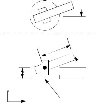
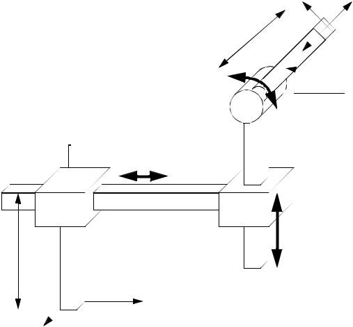
3. Robotics and Automated Manipulators (RAM) has consulted you about a new robotic manipulator. This work will include kinematic analysis, gears, and the tool. The robot is pictured below. The robot is shown on the next page in the undeformed position. The tool is a gripper (finger) type mechanism.
Tool
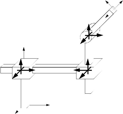
The robot is drawn below in the undeformed position. The three positioning joints are shown, and a frame at the base and tool are also shown.

page 378
|
|
|
θ |
1 |
|
|
|
x0 |
|
|
yT |
|
|
|
a |
|
|
|
|
|
|
|
|
|
z0 |
|
|
|
zT |
|
|
|
|
|
|
|
|
|
|
θ |
2 |
|
|
|
|
|
zT |
c |
|
b |
r |
|
xT |
|
|
|
|
|
|
|
y0 |
x0 |
|
|
|
|
|
|
|
|
yT xT
y0 |
z0 |
The tool is a basic gripper mechanism, and is shown as a planar mechanism below. As the cylinder moves to the left the fingers close.
|
|
|
|
|
|
|
|
|
f |
|
|
|
|
|
|
|
|||
|
|
|
|
|
|
|
|
|
|
Finger |
|||||||||
|
|
|
|
|
|
|
|
|
|
|
|
|
|
|
|
|
|||
|
|
|
|
|
|
|
|
|
|
|
|
|
|
|
|
|
|||
|
|
|
|
|
|
|
|
|
|
|
|
|
|
|
|
|
|||
|
|
|
|
|
|
|
|
|
|
|
|
|
|
|
|
|
|
|
|
|
|
|
|
|
|
|
|
|
|
|
|
|
|
|
|
|
|
|
|
|
|
|
|
|
|
|
|
|
|
|
|
|
|
|
|
|
|
|
|
Pneumatic |
|
|
|
|
|
|
|
|
|
|
|
|
|
|
|
|
|
d |
|
|
|
|
|
|
|
|
|
|
|
|
|
|
|
|
|
|
|||
|
|
|
|
|
|
|
|
|
|
|
|
|
|
|
|
|
|
|
|
cylinder |
|
|
|
|
|
|
|
|
|
|
|
|
|
|
|
|
|
e |
|
|
|
|
|
|
|
|
|
|
|
|
|
|
|
|
|
|
|
||
|
|
|
|
|
|
|
|
|
|
|
|
|
|
|
|
|
|
|
|
|
|
|
|
|
|
|
|
|
|
|
|
|
|
|
|
|
|
|
|
|
|
|
|
|
|
|
|
|
|
|
|
|
|
|
|
|
|
|
|
|
|
|
|
|
|
|
|
|
|
|
|
|
|
|
|
|
|
|
|
|
|
|
|
|
|
|
|
|
|
g |
|||||||||
|
|
|
|
|
|
|
|
|
|
|
|
|
|
|
|
|
|
|
|
|
|
|
|
|
|
|
|
|
|
|
|
|
|
|
|
|
|
|
|
|
|
|
|
|
|
|
|
|
|
|
|
|
|
|
|
|
|
|
|
|
|
|
|
|
|
|
|
|
|
|
|
|
|
|
|
|
|
|
|
a) The first thing you do is determine what sequence of rotations and translations are needed to find the tool position relative to the base position.
page 379
b)As normal, you decide to relate a cartesian (x-y) velocity of the gripper to joint velocities. Set up the calculation steps needed to do this based on the results in question #1.
c)To drive the revolute joints RAM has already selected two similar motors that have a maximum velocity. You decide to use the equations in question #2, with maximum specified tool velocities to find maximum joint velocities. Assume that helical gears are to be used to drive the revolute joints, specify the basic dimensions (such as base circle dia.). List the steps to develop the geometry of the gears, including equations.
d)The gripper fingers may close quickly, and as a result a dynamic analysis is deemed necessary. List the steps required to do an analysis (including equations) to find the dynamic forces on the fingers.
e)The idea of using a cam as an alternate mechanism is being considered. Develop a design that is equivalent to the previous design. Sketch the mechanism and a detailed displacement graph of the cam.
f)The sliding joint ‘r’ has not been designed yet. RAM wants to drive the linear motion, without using a cylinder. Suggest a reasonable design, and sketch.
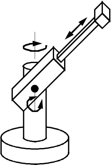
4.For an articulated robot, find the forward, and inverse kinematics using geometry, homogenous matrices, and Denavit-Hartenberg transformations.
5.Assign Denavit-Hartenberg link parameters to an articulated robot.

page 380
6. For the Stanford arm below,
θ 1
TOP VIEW
r
TCP
θ 2
d1
y
(0,0,0)
z
x
FRONT VIEW
a)list the D-H parameters (Hint: extra “dummy” joints may be required)
b)Find the forward kinematics using homogenous matrices.
c)Find the Jacobian matrix for the arm.
d)If the arm is at θ 1 = 45 degrees, θ 2 = 45 degrees, r = 0.5m, find the speed of the TCP if
the joint velocities are θ ’1 = 1 degree/sec, θ ’2 = 10 degrees/sec, and r’ = 0.01 m/ sec.
7. Consider the forward kinematic transformation of the two link manipulator below. Given the position of the joints, and the lengths of the links, determine the location of the tool centre point using a) basic geometry, b) homogenous transforms, and c) Denavit-Hartenberg transformations.

page 381
Pw(x, y)
L2 = 10” |
theta2 = 45 deg. |
|
L1 = 12” |
y |
x
theta1 = 30 deg.
a)For the robot described in question 1 determine the inverse kinematics for the robot. (i.e., given the position of the tool, determine the joint angles of the robot.) Keep in mind that in this case the solution will have two different cases. Determine two different sets of joint angles required to position the TCP at x=5”, y=6”.
b)For the inverse kinematics of question #2, what conditions would indicate the robot position is unreachable? Are there any other cases that are indeterminate?
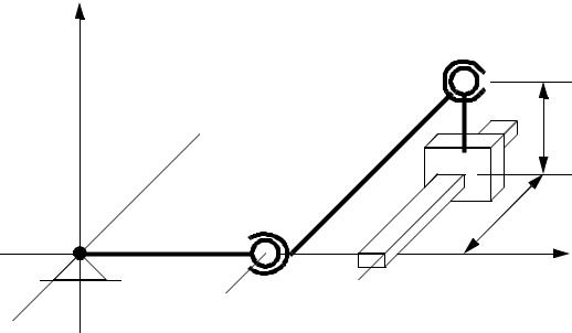
8 Find the dynamic forces in the system below,

page 382
y |
AB rotates 20rad/s c.c.w. in the |
|
|
xy plane, there are ball joints |
|
|
at B and C, and the collar at D |
C |
|
slides along the prismatic |
|
|
shaft. What are the positions, |
|
|
velocities and accelerations of |
|
|
the links? |
3” |
|
|
D |
A |
|
B |
|
|
40” |
6” |
|
|
E |
||
|
|
x |
|||
|
|
|
|||
|
|
|
|
|
|
|
|
|
|
|
|
10”
z
9.Examine the robot figure below and,
a) assign frames to the appropriate joints.

page 383
x |
z |
L4
y
θ 1
y
l2
l3
L1
x
z

page 384
ANS. |
x |
z |
|
|
|
|
|
FT |
y
|
|
y |
|
|
F3 |
|
|
x |
|
|
z |
|
y |
|
F1 |
y |
x |
|
|
|
|
x |
y |
z |
|
z |
|
|
F2 |
F0
x
z
b)list the transformations for the forward kinematics.
ans. |
= trans( 0, L1, 0) |
||
T0, 1 |
|||
T1, 2 |
= trans( l2, |
0, |
0) rot( z, 90° ) |
T2, 3 |
= trans( l3, |
0, |
0) rot( z, – 90° + θ 1) |
T3, T |
= trans( L4, 0, 0) rot( z, 90° ) rot( x, 90° ) |
c) expand the transformations to matrices (do not multiply).

page 385
ans. |
|
|
|
|
|
|
|
|
|
|
|
|
|
|
|
|
|
|
|
|
|
|
|
|
|
|
|
1 0 |
0 |
0 |
|
|
|
|
|
|
|
|
|
|
|
|
|
|
|
|
|
|
|
||||
|
|
|
|
|
|
|
|
|
|
|
|
|
|
|
|
|
|
|
|
|
||||||
|
T0, 1 = |
0 1 |
0 |
L1 |
|
|
|
|
|
|
|
|
|
|
|
|
|
|
|
|
|
|
||||
|
0 0 |
1 |
0 |
|
|
|
|
|
|
|
|
|
|
|
|
|
|
|
|
|
|
|
||||
|
|
|
|
|
|
|
|
|
|
|
|
|
|
|
|
|
|
|
|
|
||||||
|
|
0 0 |
0 |
1 |
|
|
|
|
|
|
|
|
|
|
|
|
|
|
|
|
|
|
|
|||
|
|
|
|
|
|
|
|
|
|
|
|
|
|
|
|
|
|
|
|
|
|
|
|
|
|
|
|
|
1 0 |
0 |
l2 |
cos 90° sin 90° |
0 0 |
|
|
|
|
|
|
|
|
|
|
|
|||||||||
|
T1, 2 = |
0 1 |
0 |
0 |
|
– sin 90° |
cos 90° |
0 0 |
|
|
|
|
|
|
|
|
|
|
|
|||||||
|
0 0 |
1 |
0 |
|
0 |
|
0 |
|
1 0 |
|
|
|
|
|
|
|
|
|
|
|
||||||
|
|
|
|
|
|
|
|
|
|
|
|
|
|
|
|
|||||||||||
|
|
0 0 |
0 |
1 |
|
0 |
|
0 |
|
0 1 |
|
|
|
|
|
|
|
|
|
|
|
|||||
|
|
|
|
|
|
|
|
|
|
|
|
|
|
|
|
|
|
|
|
|
|
|
|
|
|
|
|
|
|
|
|
|
|
|
|
cos ( – 90° |
+ θ |
1) |
sin ( – 90° |
+ θ |
1) |
|
|
|
|
|
|||||||
|
|
|
|
|
|
|
|
|
|
|
|
|||||||||||||||
|
|
1 0 |
0 |
l3 |
0 0 |
|
|
|
||||||||||||||||||
|
T2, 3 = |
0 1 0 0 |
– sin ( – 90° |
+ θ |
1) |
cos ( – 90° |
+ θ |
1) |
0 0 |
|
|
|
||||||||||||||
|
|
0 0 |
1 |
0 |
|
0 |
|
|
|
|
|
|
0 |
|
|
1 0 |
|
|
|
|||||||
|
|
0 0 |
0 |
1 |
|
0 |
|
|
|
|
|
|
0 |
|
|
0 1 |
|
|
|
|||||||
|
|
|
|
|
|
|
|
|
|
|
|
|
|
|
|
|
|
|
||||||||
|
|
|
|
|
|
|
|
|
|
|
|
|
|
|
|
|||||||||||
|
|
1 0 0 L4 |
|
cos 90° sin 90° |
0 0 |
|
1 |
0 |
|
0 |
0 |
|||||||||||||||
|
T3, T = |
0 1 0 |
0 |
|
– sin 90° |
cos 90° |
0 0 |
|
0 cos 90° |
sin 90° |
0 |
|||||||||||||||
|
0 0 1 |
0 |
|
0 |
|
0 |
|
1 0 |
|
0 – sin 90° |
cos 90° |
0 |
||||||||||||||
|
|
|
|
|
|
|||||||||||||||||||||
|
|
0 0 0 |
1 |
|
0 |
|
0 |
|
0 1 |
|
0 |
0 |
|
0 |
1 |
|||||||||||
|
|
|
|
|
|
|
|
|
|
|
|
|
|
|
|
|
|
|
|
|
|
|
|
|
|
|
10. Given the transformation matrix below for a polar robot,
|
|
cos ( θ ) |
sin ( θ ) 0 |
r cos ( θ ) |
||
T0, T = |
– sin ( θ ) |
cos ( θ ) |
0 |
r sin ( θ ) |
||
0 |
0 |
1 |
0 |
|||
|
||||||
|
|
0 |
0 |
0 |
1 |
a) find the Jacobian matrix.
page 386
ans. |
|
|
|
|
|
|
|
|
|
|
|
|
|
|
|
|
|
|
|
|
|
|
|
d |
|
∂ x ∂ x |
|
|
d |
|
|
|
|
|
|
|
|
|
d |
|
|
||||
|
|
|
|
|
|
|
|
|
|
|
|
|
|
|
|
|||||||
|
----x |
|
∂ r ∂ θ |
|
|
----r |
|
cos ( θ ) |
–r sin ( θ ) |
|
|
|
----r |
|||||||||
|
dt |
= |
|
|
dt |
|
|
= |
|
|
|
dt |
|
|
||||||||
|
|
d |
|
∂ y ∂ y |
|
|
d |
θ |
|
|
sin ( θ ) |
r cos ( θ ) |
|
|
|
d |
θ |
|||||
|
----y |
|
|
---- |
|
|
|
|
|
|
---- |
|||||||||||
|
|
|
|
|
|
|
|
|||||||||||||||
|
dt |
|
∂ r ∂ θ |
|
dt |
|
|
|
|
|
|
|
|
dt |
|
|
||||||
|
|
|
|
|
|
|
|
|
|
|
|
|
|
|
|
|
|
|
|
|
|
|
b) Given the joint positions, find the forward and inverse Jacobian matrices.
θ = 30° |
r = 3in |
ans. |
|
|
|
|
|
|
|
|
|
|
|
|
|
|
|
|
|
|
|
cos ( 30° ) |
–3 sin ( 30° ) |
|
|
0.866 |
–1.5 |
||||||||
J = |
|
|
|
= |
||||||||||||
|
|
|
|
|
sin ( 30° ) |
3 cos ( 30° ) |
|
|
0.5 |
2.598 |
||||||
|
|
|
|
|
|
|
|
|
|
|
|
|
|
|
|
|
J |
–1 |
= |
|
|
0.866 |
0.5 |
|
|
|
|
|
|
|
|
||
|
|
|
–0.167 0.289 |
|
|
|
|
|
|
|
||||||
|
|
|
|
|
|
|
|
|
|
|
|
|
||||
|
|
|
|
|
|
|
|
|
|
|
|
|
|
|
|
|
c) If we are at the position below, and want to move the tool at the given speed, what joint
velocities are required?
d |
in |
d |
in |
----x = –1---- |
----y = 2---- |
||
dt |
s |
dt |
s |
ans. |
|
d |
|
|
|
|
|
|
|
|
|
|
|
|
|
|
|
|
|
|
|
|
|
|
|
|
|
|
|
|
|
||
|
|
|
|
|
|
|
|
|
|
|
|
|
|
|
|
|
|
|
----r |
|
0.866 0.5 |
|
|
–1 |
|
0.134 |
|||||||
|
|
dt |
|
|
= |
|
|
= |
||||||||
|
|
d |
|
–0.167 0.289 |
|
2 |
|
0.745 |
||||||||
|
|
θ |
|
|
|
|
||||||||||
|
---- |
|
|
|
|
|
|
|
|
|
|
|
|
|||
|
|
|
|
|
|
|
|
|
|
|
|
|
||||
|
dt |
|
|
|
|
|
|
|
|
|
|
|
|
|
|
|
|
|
|
|
|
|
|
|
|
|
|
|
|
|
|
|
|
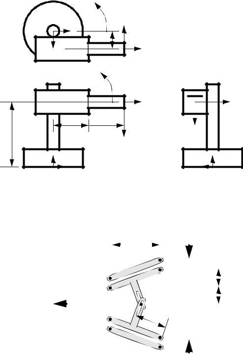
11. Examine the robot figure below and,
a) assign frames to the appropriate joints.

page 387
|
|
|
θ |
1 |
|
|
|
x0 |
|
|
xT |
|
|
|
a |
|
|
|
|
|
|
|
|
|
z0 |
|
|
|
zT |
|
|
|
|
|
yT |
|
|
|
|
θ |
yT |
|
|
|
|
2 |
|
|
|
|
|
|
zT |
|
|
|
|
|
xT |
c |
|
b |
r |
|
|
|
y0 |
x0 |
|
|
y0 |
|
|
|
|
z0 |
b)list the transformations for the forward kinematics.
c)expand the transformations to matrices (do not multiply).
12. Given the transformation matrix below for a polar robot,
|
|
cos ( θ 1 + θ 2) |
sin ( θ 1 + θ 2) |
0 |
cos θ |
1 |
+ 1.2 cos ( θ |
1 + θ |
2) |
T0, T = |
– sin ( θ 1 + θ 2) |
cos ( θ 1 + θ 2) |
0 |
sin θ |
1 |
+ 1.2 sin ( θ |
1 + θ |
2) |
|
|
0 |
0 |
1 |
|
|
0 |
|
|
|
|
|
0 |
0 |
0 |
|
|
1 |
|
|
a)find the Jacobian matrix.
b)Given the joint positions, find the forward and inverse Jacobian matrices.
θ 1 = 30° |
θ 1 = 40° |
c) If we are at the position below, and want to move the tool at the given speed, what joint velocities are required?

page 388
d |
in |
d |
in |
----x = –1---- |
----y = 2---- |
||
dt |
s |
dt |
s |
13. Find the forward kinematics for the robots below using homogeneous and DenavitHartenberg matrices.
y |
y |
y |
|
x |
|
|
|
|
|
|
|
|
|
|
|
x |
|
|
|
x |
||
|
|
|
|
|
|
|
|||
y |
|
|
|
y |
|
|
|
|
|
|
|
|
|
x |
|
|
x |
|
|
14. Use the equations below to find the inverse Jacobian. Use the inverse Jacobian to find the joint velocities required at t=0.5s.
x |
= |
4 cos ( θ |
1) |
+ 6 cos ( θ 1 + θ 2) |
in. |
y |
= |
4 sin ( θ |
1) |
+ 6 sin ( θ 1 + θ 2) |
in. |

page 389
ANS.
First, find tool and joint positions, |
|
|
|
|
|
|
|
|
|
|
|
|
|
|
|
|
|
|
|
|
||||||||||||||||||
|
|
|
|
|
|
|
|
|
|
|
|
|
|
|
|
|
|
|
|
|
|
|
|
|
|
|
|
|
|
|
|
|
||||||
P( 0.5) |
= |
|
3 |
|
+ ( – 2t3 + 3t2) |
5 |
|
= |
|
5.5 |
|
|
|
|
|
|
|
|
|
|
|
|
||||||||||||||||
|
|
|
|
|
|
|
|
|
|
5 |
|
|
|
|
|
|
|
2 |
|
|
|
6 |
|
|
|
|
|
|
|
|
|
|
|
|
|
|||
|
|
|
|
|
|
|
|
|
|
|
|
|
|
|
|
|
|
|
|
|
|
|
|
|
|
|
|
|
|
|
|
|
|
|
|
|
|
|
r |
|
= |
|
5.5 |
2 |
+ 6 |
2 |
|
|
α |
= |
|
|
|
|
|
6 |
|
|
|
|
|
|
|
|
|
|
|
||||||||||
|
|
|
|
|
|
|
atan |
------ |
|
|
|
|
|
|
|
|
|
|
|
|
|
|||||||||||||||||
|
|
|
|
|
|
|
|
|
|
|
|
|
|
|
|
|
|
|
|
|
|
|
5.5 |
|
|
|
|
|
|
|
|
|
r2 – ( 42 + 62) |
|||||
|
2 |
|
|
|
|
|
2 |
|
|
2 |
|
|
|
|
|
|
|
|
|
|
· |
2) |
· |
θ |
|
|
|
|
|
|||||||||
r |
|
= 4 |
|
+ 6 |
|
|
– 2( 4) ( 6) cos ( 180 – θ |
|
2 |
= 180 – acos --------------------------------–2( 4) ( 6) |
|
|||||||||||||||||||||||||||
sin ( θ |
1 – α ) |
= |
|
sin ( 180 – θ 2) |
|
|
|
|
|
|
|
|
· |
θ |
1 |
= asin |
|
6 sin ( 180 – θ 2) |
+ α |
|
||||||||||||||||||
--------------------------- |
|
|
|
|
6 |
|
|
|
|
-------------------------------- |
|
|
r |
|
|
|
|
|
|
|
|
|
|
------------------------------------r |
|
|
||||||||||||
|
|
|
|
|
|
|
|
|
|
|
|
|
|
|
|
|
|
|
|
|
|
|
|
|
|
|
|
|
|
|
|
|
||||||
|
|
|
|
|
|
|
|
|
|
|
|
|
|
|
|
|
|
|
|
|
|
|
|
|
|
|
|
|
|
|
|
|
|
|
||||
Next, the Jacobian, |
|
|
|
|
|
|
|
|
|
|
|
|
|
|
|
|
|
|
|
|
|
|
|
|
|
|
|
|
|
|||||||||
|
|
|
|
|
|
|
|
|
|
|
|
|
|
|
|
|
|
|
|
|
||||||||||||||||||
J |
= |
|
– 4 sin ( θ |
1) |
|
– 6 sin ( θ |
1 + θ 2) |
–6 sin ( θ |
1 + θ 2) |
|
|
|
|
|
|
|||||||||||||||||||||||
|
|
|
|
|
|
4 cos ( θ |
1) |
+ 6 cos ( θ |
1 + θ |
2) |
6 cos ( θ |
1 + θ |
2) |
|
|
|
|
|
|
|
||||||||||||||||||
Substitute and solve |
|
|
|
|
|
|
|
|
|
|
|
|
|
|
|
|
|
|
|
|
|
|
|
|
|
|
|
|||||||||||
|
|
|
|
|
|
|
|
|
|
|
|
|
|
|
|
|
|
|
|
|
|
|
|
|
|
|
|
|
|
|
|
|
|
|
|
|
||
d |
|
θ |
1 |
|
= |
J |
–1 |
|
7.5 |
|
|
|
|
|
|
|
|
|
|
|
|
|
|
|
|
|
|
|
|
|
|
|||||||
---- |
|
|
|
|
|
|
|
|
|
|
|
|
|
|
|
|
|
|
|
|
|
|
|
|
|
|
|
|
|
|||||||||
dt |
|
θ 2 |
|
|
|
|
|
|
|
3 |
|
|
|
|
|
|
|
|
|
|
|
|
|
|
|
|
|
|
|
|
|
|
|
|||||
|
|
|
|
|
|
|
|
|
|
|
|
|
|
|
|
|
|
|
|
|
|
|
|
|
|
|
|
|
|
|
|
|
|
|
|
|||
|
|
|
|
|
|
|
|
|
|
|
|
|
|
|
|
|
|
|
|
|
|
|
|
|
|
|
|
|
|
|
|
|
|
|
|
|
|
|