

- •1. INTEGRATED AND AUTOMATED MANUFACTURING
- •1.1 INTRODUCTION
- •1.1.1 Why Integrate?
- •1.1.2 Why Automate?
- •1.2 THE BIG PICTURE
- •1.2.2 The Architecture of Integration
- •1.2.3 General Concepts
- •1.3 PRACTICE PROBLEMS
- •2. AN INTRODUCTION TO LINUX/UNIX
- •2.1 OVERVIEW
- •2.1.1 What is it?
- •2.1.2 A (Brief) History
- •2.1.3 Hardware required and supported
- •2.1.4 Applications and uses
- •2.1.5 Advantages and Disadvantages
- •2.1.6 Getting It
- •2.1.7 Distributions
- •2.1.8 Installing
- •2.2 USING LINUX
- •2.2.1 Some Terminology
- •2.2.2 File and directories
- •2.2.3 User accounts and root
- •2.2.4 Processes
- •2.3 NETWORKING
- •2.3.1 Security
- •2.4 INTERMEDIATE CONCEPTS
- •2.4.1 Shells
- •2.4.2 X-Windows
- •2.4.3 Configuring
- •2.4.4 Desktop Tools
- •2.5 LABORATORY - A LINUX SERVER
- •2.6 TUTORIAL - INSTALLING LINUX
- •2.7 TUTORIAL - USING LINUX
- •2.8 REFERENCES
- •3. AN INTRODUCTION TO C/C++ PROGRAMMING
- •3.1 INTRODUCTION
- •3.2 PROGRAM PARTS
- •3.3 CLASSES AND OVERLOADING
- •3.4 HOW A ‘C’ COMPILER WORKS
- •3.5 STRUCTURED ‘C’ CODE
- •3.6 COMPILING C PROGRAMS IN LINUX
- •3.6.1 Makefiles
- •3.7 ARCHITECTURE OF ‘C’ PROGRAMS (TOP-DOWN)
- •3.8 CREATING TOP DOWN PROGRAMS
- •3.9 CASE STUDY - THE BEAMCAD PROGRAM
- •3.9.1 Objectives:
- •3.9.2 Problem Definition:
- •3.9.3 User Interface:
- •3.9.3.1 - Screen Layout (also see figure):
- •3.9.3.2 - Input:
- •3.9.3.3 - Output:
- •3.9.3.4 - Help:
- •3.9.3.5 - Error Checking:
- •3.9.3.6 - Miscellaneous:
- •3.9.4 Flow Program:
- •3.9.5 Expand Program:
- •3.9.6 Testing and Debugging:
- •3.9.7 Documentation
- •3.9.7.1 - Users Manual:
- •3.9.7.2 - Programmers Manual:
- •3.9.8 Listing of BeamCAD Program.
- •3.10 PRACTICE PROBLEMS
- •3.11 LABORATORY - C PROGRAMMING
- •4. NETWORK COMMUNICATION
- •4.1 INTRODUCTION
- •4.2 NETWORKS
- •4.2.1 Topology
- •4.2.2 OSI Network Model
- •4.2.3 Networking Hardware
- •4.2.4 Control Network Issues
- •4.2.5 Ethernet
- •4.2.6 SLIP and PPP
- •4.3 INTERNET
- •4.3.1 Computer Addresses
- •4.3.2 Computer Ports
- •4.3.2.1 - Mail Transfer Protocols
- •4.3.2.2 - FTP - File Transfer Protocol
- •4.3.2.3 - HTTP - Hypertext Transfer Protocol
- •4.3.3 Security
- •4.3.3.1 - Firewalls and IP Masquerading
- •4.4 FORMATS
- •4.4.1 HTML
- •4.4.2 URLs
- •4.4.3 Encryption
- •4.4.4 Clients and Servers
- •4.4.5 Java
- •4.4.6 Javascript
- •4.5 NETWORKING IN LINUX
- •4.5.1 Network Programming in Linux
- •4.6 DESIGN CASES
- •4.7 SUMMARY
- •4.8 PRACTICE PROBLEMS
- •4.9 LABORATORY - NETWORKING
- •4.9.1 Prelab
- •4.9.2 Laboratory
- •5. DATABASES
- •5.1 SQL AND RELATIONAL DATABASES
- •5.2 DATABASE ISSUES
- •5.3 LABORATORY - SQL FOR DATABASE INTEGRATION
- •5.4 LABORATORY - USING C FOR DATABASE CALLS
- •6. COMMUNICATIONS
- •6.1 SERIAL COMMUNICATIONS
- •6.2 SERIAL COMMUNICATIONS UNDER LINUX
- •6.3 PARALLEL COMMUNICATIONS
- •6.4 LABORATORY - SERIAL INTERFACING AND PROGRAMMING
- •6.5 LABORATORY - STEPPER MOTOR CONTROLLER
- •7. PROGRAMMABLE LOGIC CONTROLLERS (PLCs)
- •7.1 BASIC LADDER LOGIC
- •7.2 WHAT DOES LADDER LOGIC DO?
- •7.2.1 Connecting A PLC To A Process
- •7.2.2 PLC Operation
- •7.3 LADDER LOGIC
- •7.3.1 Relay Terminology
- •7.3.2 Ladder Logic Inputs
- •7.3.3 Ladder Logic Outputs
- •7.4 LADDER DIAGRAMS
- •7.4.1 Ladder Logic Design
- •7.4.2 A More Complicated Example of Design
- •7.5 TIMERS/COUNTERS/LATCHES
- •7.6 LATCHES
- •7.7 TIMERS
- •7.8 COUNTERS
- •7.9 DESIGN AND SAFETY
- •7.9.1 FLOW CHARTS
- •7.10 SAFETY
- •7.10.1 Grounding
- •7.10.2 Programming/Wiring
- •7.10.3 PLC Safety Rules
- •7.10.4 Troubleshooting
- •7.11 DESIGN CASES
- •7.11.1 DEADMAN SWITCH
- •7.11.2 CONVEYOR
- •7.11.3 ACCEPT/REJECT SORTING
- •7.11.4 SHEAR PRESS
- •7.12 ADDRESSING
- •7.12.1 Data Files
- •7.12.1.1 - Inputs and Outputs
- •7.12.1.2 - User Numerical Memory
- •7.12.1.3 - Timer Counter Memory
- •7.12.1.4 - PLC Status Bits (for PLC-5s)
- •7.12.1.5 - User Function Memory
- •7.13 INSTRUCTION TYPES
- •7.13.1 Program Control Structures
- •7.13.2 Branching and Looping
- •7.13.2.1 - Immediate I/O Instructions
- •7.13.2.2 - Fault Detection and Interrupts
- •7.13.3 Basic Data Handling
- •7.13.3.1 - Move Functions
- •7.14 MATH FUNCTIONS
- •7.15 LOGICAL FUNCTIONS
- •7.15.1 Comparison of Values
- •7.16 BINARY FUNCTIONS
- •7.17 ADVANCED DATA HANDLING
- •7.17.1 Multiple Data Value Functions
- •7.17.2 Block Transfer Functions
- •7.18 COMPLEX FUNCTIONS
- •7.18.1 Shift Registers
- •7.18.2 Stacks
- •7.18.3 Sequencers
- •7.19 ASCII FUNCTIONS
- •7.20 DESIGN TECHNIQUES
- •7.20.1 State Diagrams
- •7.21 DESIGN CASES
- •7.21.1 If-Then
- •7.21.2 For-Next
- •7.21.3 Conveyor
- •7.22 IMPLEMENTATION
- •7.23 PLC WIRING
- •7.23.1 SWITCHED INPUTS AND OUTPUTS
- •7.23.1.1 - Input Modules
- •7.23.1.2 - Actuators
- •7.23.1.3 - Output Modules
- •7.24 THE PLC ENVIRONMENT
- •7.24.1 Electrical Wiring Diagrams
- •7.24.2 Wiring
- •7.24.3 Shielding and Grounding
- •7.24.4 PLC Environment
- •7.24.5 SPECIAL I/O MODULES
- •7.25 PRACTICE PROBLEMS
- •7.26 REFERENCES
- •7.27 LABORATORY - SERIAL INTERFACING TO A PLC
- •8. PLCS AND NETWORKING
- •8.1 OPEN NETWORK TYPES
- •8.1.1 Devicenet
- •8.1.2 CANbus
- •8.1.3 Controlnet
- •8.1.4 Profibus
- •8.2 PROPRIETARY NETWORKS
- •8.2.0.1 - Data Highway
- •8.3 PRACTICE PROBLEMS
- •8.4 LABORATORY - DEVICENET
- •8.5 TUTORIAL - SOFTPLC AND DEVICENET
- •9. INDUSTRIAL ROBOTICS
- •9.1 INTRODUCTION
- •9.1.1 Basic Terms
- •9.1.2 Positioning Concepts
- •9.1.2.1 - Accuracy and Repeatability
- •9.1.2.2 - Control Resolution
- •9.1.2.3 - Payload
- •9.2 ROBOT TYPES
- •9.2.1 Basic Robotic Systems
- •9.2.2 Types of Robots
- •9.2.2.1 - Robotic Arms
- •9.2.2.2 - Autonomous/Mobile Robots
- •9.2.2.2.1 - Automatic Guided Vehicles (AGVs)
- •9.3 MECHANISMS
- •9.4 ACTUATORS
- •9.5 A COMMERCIAL ROBOT
- •9.5.1 Mitsubishi RV-M1 Manipulator
- •9.5.2 Movemaster Programs
- •9.5.2.0.1 - Language Examples
- •9.5.3 Command Summary
- •9.6 PRACTICE PROBLEMS
- •9.7 LABORATORY - MITSUBISHI RV-M1 ROBOT
- •9.8 TUTORIAL - MITSUBISHI RV-M1
- •10. OTHER INDUSTRIAL ROBOTS
- •10.1 SEIKO RT 3000 MANIPULATOR
- •10.1.1 DARL Programs
- •10.1.1.1 - Language Examples
- •10.1.1.2 - Commands Summary
- •10.2 IBM 7535 MANIPULATOR
- •10.2.1 AML Programs
- •10.3 ASEA IRB-1000
- •10.4 UNIMATION PUMA (360, 550, 560 SERIES)
- •10.5 PRACTICE PROBLEMS
- •10.6 LABORATORY - SEIKO RT-3000 ROBOT
- •10.7 TUTORIAL - SEIKO RT-3000 ROBOT
- •10.8 LABORATORY - ASEA IRB-1000 ROBOT
- •10.9 TUTORIAL - ASEA IRB-1000 ROBOT
- •11. ROBOT APPLICATIONS
- •11.0.1 Overview
- •11.0.2 Spray Painting and Finishing
- •11.0.3 Welding
- •11.0.4 Assembly
- •11.0.5 Belt Based Material Transfer
- •11.1 END OF ARM TOOLING (EOAT)
- •11.1.1 EOAT Design
- •11.1.2 Gripper Mechanisms
- •11.1.2.1 - Vacuum grippers
- •11.1.3 Magnetic Grippers
- •11.1.3.1 - Adhesive Grippers
- •11.1.4 Expanding Grippers
- •11.1.5 Other Types Of Grippers
- •11.2 ADVANCED TOPICS
- •11.2.1 Simulation/Off-line Programming
- •11.3 INTERFACING
- •11.4 PRACTICE PROBLEMS
- •11.5 LABORATORY - ROBOT INTERFACING
- •11.6 LABORATORY - ROBOT WORKCELL INTEGRATION
- •12. SPATIAL KINEMATICS
- •12.1 BASICS
- •12.1.1 Degrees of Freedom
- •12.2 HOMOGENEOUS MATRICES
- •12.2.1 Denavit-Hartenberg Transformation (D-H)
- •12.2.2 Orientation
- •12.2.3 Inverse Kinematics
- •12.2.4 The Jacobian
- •12.3 SPATIAL DYNAMICS
- •12.3.1 Moments of Inertia About Arbitrary Axes
- •12.3.2 Euler’s Equations of Motion
- •12.3.3 Impulses and Momentum
- •12.3.3.1 - Linear Momentum
- •12.3.3.2 - Angular Momentum
- •12.4 DYNAMICS FOR KINEMATICS CHAINS
- •12.4.1 Euler-Lagrange
- •12.4.2 Newton-Euler
- •12.5 REFERENCES
- •12.6 PRACTICE PROBLEMS
- •13. MOTION CONTROL
- •13.1 KINEMATICS
- •13.1.1 Basic Terms
- •13.1.2 Kinematics
- •13.1.2.1 - Geometry Methods for Forward Kinematics
- •13.1.2.2 - Geometry Methods for Inverse Kinematics
- •13.1.3 Modeling the Robot
- •13.2 PATH PLANNING
- •13.2.1 Slew Motion
- •13.2.1.1 - Joint Interpolated Motion
- •13.2.1.2 - Straight-line motion
- •13.2.2 Computer Control of Robot Paths (Incremental Interpolation)
- •13.3 PRACTICE PROBLEMS
- •13.4 LABORATORY - AXIS AND MOTION CONTROL
- •14. CNC MACHINES
- •14.1 MACHINE AXES
- •14.2 NUMERICAL CONTROL (NC)
- •14.2.1 NC Tapes
- •14.2.2 Computer Numerical Control (CNC)
- •14.2.3 Direct/Distributed Numerical Control (DNC)
- •14.3 EXAMPLES OF EQUIPMENT
- •14.3.1 EMCO PC Turn 50
- •14.3.2 Light Machines Corp. proLIGHT Mill
- •14.4 PRACTICE PROBLEMS
- •14.5 TUTORIAL - EMCO MAIER PCTURN 50 LATHE (OLD)
- •14.6.1 LABORATORY - CNC MACHINING
- •15. CNC PROGRAMMING
- •15.1 G-CODES
- •15.3 PROPRIETARY NC CODES
- •15.4 GRAPHICAL PART PROGRAMMING
- •15.5 NC CUTTER PATHS
- •15.6 NC CONTROLLERS
- •15.7 PRACTICE PROBLEMS
- •15.8 LABORATORY - CNC INTEGRATION
- •16. DATA AQUISITION
- •16.1 INTRODUCTION
- •16.2 ANALOG INPUTS
- •16.3 ANALOG OUTPUTS
- •16.4 REAL-TIME PROCESSING
- •16.5 DISCRETE IO
- •16.6 COUNTERS AND TIMERS
- •16.7 ACCESSING DAQ CARDS FROM LINUX
- •16.8 SUMMARY
- •16.9 PRACTICE PROBLEMS
- •16.10 LABORATORY - INTERFACING TO A DAQ CARD
- •17. VISIONS SYSTEMS
- •17.1 OVERVIEW
- •17.2 APPLICATIONS
- •17.3 LIGHTING AND SCENE
- •17.4 CAMERAS
- •17.5 FRAME GRABBER
- •17.6 IMAGE PREPROCESSING
- •17.7 FILTERING
- •17.7.1 Thresholding
- •17.8 EDGE DETECTION
- •17.9 SEGMENTATION
- •17.9.1 Segment Mass Properties
- •17.10 RECOGNITION
- •17.10.1 Form Fitting
- •17.10.2 Decision Trees
- •17.11 PRACTICE PROBLEMS
- •17.12 TUTORIAL - LABVIEW BASED IMAQ VISION
- •17.13 LABORATORY - VISION SYSTEMS FOR INSPECTION
- •18. INTEGRATION ISSUES
- •18.1 CORPORATE STRUCTURES
- •18.2 CORPORATE COMMUNICATIONS
- •18.3 COMPUTER CONTROLLED BATCH PROCESSES
- •18.4 PRACTICE PROBLEMS
- •18.5 LABORATORY - WORKCELL INTEGRATION
- •19. MATERIAL HANDLING
- •19.1 INTRODUCTION
- •19.2 VIBRATORY FEEDERS
- •19.3 PRACTICE QUESTIONS
- •19.4 LABORATORY - MATERIAL HANDLING SYSTEM
- •19.4.1 System Assembly and Simple Controls
- •19.5 AN EXAMPLE OF AN FMS CELL
- •19.5.1 Overview
- •19.5.2 Workcell Specifications
- •19.5.3 Operation of The Cell
- •19.6 THE NEED FOR CONCURRENT PROCESSING
- •19.7 PRACTICE PROBLEMS
- •20. PETRI NETS
- •20.1 INTRODUCTION
- •20.2 A BRIEF OUTLINE OF PETRI NET THEORY
- •20.3 MORE REVIEW
- •20.4 USING THE SUBROUTINES
- •20.4.1 Basic Petri Net Simulation
- •20.4.2 Transitions With Inhibiting Inputs
- •20.4.3 An Exclusive OR Transition:
- •20.4.4 Colored Tokens
- •20.4.5 RELATIONAL NETS
- •20.5 C++ SOFTWARE
- •20.6 IMPLEMENTATION FOR A PLC
- •20.7 PRACTICE PROBLEMS
- •20.8 REFERENCES
- •21. PRODUCTION PLANNING AND CONTROL
- •21.1 OVERVIEW
- •21.2 SCHEDULING
- •21.2.1 Material Requirements Planning (MRP)
- •21.2.2 Capacity Planning
- •21.3 SHOP FLOOR CONTROL
- •21.3.1 Shop Floor Scheduling - Priority Scheduling
- •21.3.2 Shop Floor Monitoring
- •22. SIMULATION
- •22.1 MODEL BUILDING
- •22.2 ANALYSIS
- •22.3 DESIGN OF EXPERIMENTS
- •22.4 RUNNING THE SIMULATION
- •22.5 DECISION MAKING STRATEGY
- •23. PLANNING AND ANALYSIS
- •23.1 FACTORS TO CONSIDER
- •23.2 PROJECT COST ACCOUNTING
- •24. REFERENCES
- •25. APPENDIX A - PROJECTS
- •25.1 TOPIC SELECTION
- •25.1.1 Previous Project Topics
- •25.2 CURRENT PROJECT DESCRIPTIONS
- •26. APPENDIX B - COMMON REFERENCES
- •26.1 JIC ELECTRICAL SYMBOLS
- •26.2 NEMA ENCLOSURES

page 363
• We can find these angles given a set of axis before and after.
|
|
|
|
|
|
|
|
|
|
|
|
|
x0 = |
1 |
x1 = |
0.71 |
y0 = |
|
|
|
y1 = |
||||
0 |
0.71 |
|
|
|
||||||||
|
0 |
|
0 |
|
|
|
|
|
|
|||
|
|
|
|
|
|
|
|
|
|
|
|
|
12.2.3 Inverse Kinematics
•Basically we can find the joint angles for the robot based on the position of the end effector.
•This is not a simple problem, and there are few reliable methods. This is partly caused by the non-unique nature of the problem. At best there are typically multiple, if not infinite numbers of equivalent solutions. The 2 dof robot seen before has two possible solutions.
•We can do simple inverse kinematics with trigonometry.
•If we have more complicated problems, we may try to solve the problem by examining the transform matrix,
page 364
|
|
|
|
|
|
|
|
|
|
|
|
|
|
|
|
|
|
|
|
|
|
|
|
|
|
|
|
|
|
|
|
|
|
|
|
|
|
|
|
|
|
cos ( θ 1 + θ |
2) |
|
sin ( θ |
1 + θ |
2) 0 cos θ |
1 + 1.2 cos ( θ |
1 + θ |
2) |
|
||||||||||||||||||||||||||
T0, T = |
|
– sin ( θ |
1 + θ 2) |
|
cos ( θ |
1 + θ |
2) |
0 |
|
sin θ |
1 + 1.2 sin ( θ |
1 + θ |
2) |
|
|
|||||||||||||||||||||||
|
|
|
|
|
|
0 |
|
|
|
|
|
|
|
0 |
|
|
|
|
1 |
|
|
|
|
|
|
|
|
|
0 |
|
|
|
|
|
|
|
|
|
|
|
|
|
|
|
0 |
|
|
|
|
|
|
|
0 |
|
|
|
|
0 |
|
|
|
|
|
|
|
|
|
1 |
|
|
|
|
|
|
|
|
|
Separate positions and simplify, |
|
|
|
|
|
|
|
|
|
|
|
|
|
|
|
|
|
|
|
|
|
|
|
|||||||||||||||
xT |
= |
cos θ 1 + 1.2 cos ( θ |
1 + θ |
2) |
|
|
|
|
|
|
|
|
|
|
|
|
|
|
|
|
|
|
|
|
||||||||||||||
xT |
|
– cos θ 1 |
= |
cosθ( |
|
+ θ |
2) |
|
|
|
|
|
|
|
|
|
|
|
|
|
|
|
|
|
|
|
|
|||||||||||
------------------------- |
1 |
|
|
|
|
|
|
|
|
|
|
|
|
|
|
|
|
|
|
|
|
|||||||||||||||||
|
|
|
|
|
1.2 |
|
|
|
|
|
|
|
|
|
|
|
|
|
|
|
|
|
|
|
|
|
|
|
|
|
|
|
|
|
|
|
|
|
yT |
= |
sin θ 1 + 1.2 sin ( θ |
1 + θ |
2) |
|
|
|
|
|
|
|
|
|
|
|
|
|
|
|
|
|
|
|
|
||||||||||||||
|
yT |
– sin θ 1 |
= |
sinθ( |
|
+ θ |
2) |
|
|
|
|
|
|
|
|
|
|
|
|
|
|
|
|
|
|
|
|
|||||||||||
------------------------ |
1 |
|
|
|
|
|
|
|
|
|
|
|
|
|
|
|
|
|
|
|
|
|||||||||||||||||
|
|
|
|
|
1.2 |
|
|
|
|
|
|
|
|
|
|
|
|
|
|
|
|
|
|
|
|
|
|
|
|
|
|
|
|
|
|
|
|
|
Combine the two to eliminate the compound angles, |
|
|
|
|
|
|
|
|
|
|||||||||||||||||||||||||||||
1 = ( cos ( θ |
1 |
+ θ |
2 |
) ) 2 |
+ ( sin ( θ |
1 |
+ θ |
2 |
) ) 2 |
|
|
|
|
|
|
|
|
|
|
|
||||||||||||||||||
|
|
|
|
|
|
|
|
|
|
|
|
|
|
|
|
|
|
|
|
|
|
|
|
|
|
|
|
|
|
|
|
|
|
|||||
|
1 |
= |
xT |
– cos θ |
1 2 |
|
|
yT |
– sin θ |
1 |
|
2 |
|
|
|
|
|
|
|
|
|
|
|
|
|
|||||||||||||
------------------------- |
+ |
------------------------ |
|
|
|
|
|
|
|
|
|
|
|
|
|
|
||||||||||||||||||||||
|
|
|
|
|
|
|
1.2 |
|
|
|
|
|
|
|
|
|
1.2 |
|
|
|
|
|
|
|
|
|
|
|
|
|
|
|
|
|
||||
1.44 = x2 |
– 2x |
T |
cos θ |
1 |
+ ( cos θ |
|
) |
2 + y2 |
– 2y |
T |
sin θ |
1 |
+ ( sin θ ) 2 |
|||||||||||||||||||||||||
|
|
|
|
|
|
|
T |
|
|
|
|
|
|
|
|
|
|
|
|
1 |
|
|
|
|
T |
|
|
|
|
|
1 |
|||||||
|
|
|
( 0.44 – x2 |
– x2) |
|
= – 2x |
T |
cos θ |
1 |
– 2y |
T |
sin θ |
1 |
|
|
|
|
|
|
|
|
|||||||||||||||||
|
|
|
|
|
|
|
T |
|
T |
|
|
|
|
|
|
|
|
|
|
|
|
|
|
|
|
|
|
|
|
|
|
|
|
|||||
|
|
|
|
0.44 – xT2 – xT2 |
|
= |
( xT cos θ |
1 + yT sin θ 1) |
|
|
|
|
|
|
|
|
|
|||||||||||||||||||||
|
|
|
-------------------------------- |
|
|
|
|
|
|
|
|
|
|
|||||||||||||||||||||||||
|
|
|
|
|
|
–2 |
|
|
|
|
|
|
|
|
|
|
|
|
|
|
|
|
|
|
|
|
|
|
|
|
|
|
|
|
|
|
|
|
ETC.....
12.2.4 The Jacobian
page 365
• A matrix of partial derivatives that relate the velocity of the joints, to the velocity of the
tool.
|
|
|
|
|
|
|
|
|
|
|
|
|
|
|
|
|
|
|
|
|
|
|
d |
|
|
|
∂ |
xT |
∂ |
xT |
∂ |
xT |
|
|
d |
|
|
|
|
d |
|
||
|
|
|
|
|
|
|
|
|
|
|
|||||||||||
|
T |
|
-------- |
-------- |
-------- |
|
|
1 |
|
|
θ |
||||||||||
dt |
|
∂θ |
1 |
∂θ |
2 |
∂θ |
3 |
|
dt |
|
dt |
||||||||||
----x |
|
|
|
|
|
|
|
|
|
|
|
|
---- |
θ |
|
---- |
|||||
|
d |
|
|
= |
∂ yT |
∂ yT |
∂ yT |
|
|
d |
θ |
= J |
|
d |
θ |
||||||
----y |
|
-------- |
-------- |
-------- |
|
---- |
---- |
||||||||||||||
dt |
T |
|
∂θ |
1 |
∂θ |
2 |
∂θ |
3 |
|
dt |
2 |
|
dt |
|
|||||||
|
d |
|
|
|
∂ |
zT |
∂ |
zT |
∂ |
zT |
|
|
d |
θ |
|
|
d |
θ |
|||
----z |
T |
|
|
---- |
|
---- |
|||||||||||||||
dt |
|
-------- |
-------- |
-------- |
|
dt |
3 |
|
dt |
|
|||||||||||
|
|
|
|
|
∂θ |
1 |
∂θ |
2 |
∂θ |
3 |
|
|
|
|
|
|
|
|
|
||
|
|
|
|
|
|
|
|
|
|
|
|
|
|
||||||||
|
|
|
|
|
|
|
|
|
|
|
|
|
|
|
|
|
|
|
|
|
|
• The inverse Jacobian is used for motion control
1
2
3
|
|
|
· |
|
|
|
· |
|
|
|
–1 |
xT |
|
θ |
1 |
||||
J |
· |
|
= |
· |
|
|
|||
|
yT |
θ |
2 |
||||||
|
|
· |
|
|
· |
|
|
||
|
|
zT |
|
θ |
3 |
||||
|
|
|
|
|
|
|
|
|
|
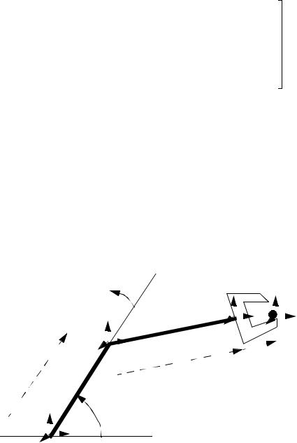
• Find the Jacobian and inverse Jacobian for the 2 dof robot.
|
|
|
θ 2 |
|
|
y |
|
y |
F |
T |
|||
|
|
|
|
|
|
|
F2 |
|
|||||
|
|
|
|
|
|
|
|
|
|
|
|
||
|
|
|
|
y |
|
|
|
xz |
|
x |
|||
|
|
|
|
|
|
|
|||||||
|
|
|
F1 |
|
z |
|
|
|
|||||
|
|
|
|
|
|
|
|||||||
|
|
|
|
|
x |
|
|
|
|
||||
|
|
|
|
|
|
|
|
||||||
|
|
|
|
|
|
|
|
|
|
||||
T0, 1 |
z |
T2, T |
|
|
|||||||||
|
|
|
|
|
|
||||||||
|
|
|
|
T1, 2 |
|
|
|||||||
|
|
|
|
|
|
|
|
|
|
|
|||
F0 |
y |
θ 1 |
|
|
|
|
|
|
|
|
|||
|
|
x |
|
|
|
|
|
|
|
|
|||
|
|
|
|
|
|
|
|
|
|||||
|
|
|
|
|
|
|
|
|
|
|
|||
z |
|
|
|
|
|
|
|
|
|||||
|
|
|
|
|
|
|
|
|
|
|
|||