page 359

• To reverse the transform, we only need to invert the transform matrix - this is a direct result of the loop equation.

T0, 1T1, 2T2, TTT, 0 = I

where,

I = Identity matrix

We can manipulate the equation,

T0, TTT, 0 = I

TT, 0 = ( T0, T) –1

12.2.1 Denavit-Hartenberg Transformation (D-H)

•Designed as more specialized transforms for robots (based on homogenous transforms)

•Zi-1 axis along motion of ith joint

•Xi axis normal to Zi-1 axis, and points away from it.

•Basic transform is,

1.rotate about Zi-1 by thetai (joint angle)

2.translate along Zi-1 by di (link offset)

3.translate along Xi by ai (link length)

4.rotate about Xi by alphai (link twist)

page 360

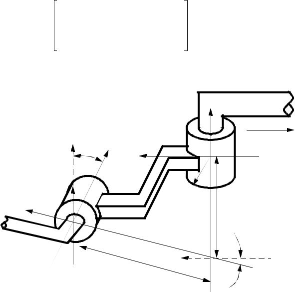
• We can see how the D-H representation is applied using the two link manipulator from before

page 362

•The main problem in representing orientation is that the angles of rotation must be applied one at a time, and by changing the sequence we will change the final orientation. In other words the three angles will not give a unique solution unless applied in the same sequence every time.

•By fixing a set of angles by convention we can then use the three angles by themselves to define an orientation.

•The convention described here is the Euler angles.

•The sequence of orientation is,

In order,

rot( θ ) , rot( φ ) , rot( ψ )

where,

θ= rotation about z axis

φ= rotation about new x axis

ψ= rotation about new z axis

•Therefore to reorient a point in space we can apply the following matrix, to the position vectors, or axes vectors, (there will be more on these matrices shortly)