

funct_a_l
.pdfExample 2: A solve block with both equations and inequalities.
Example 3: Solving an equation repeatedly (by defining the Reynolds number R to be a range variable).
Functions |
33 |
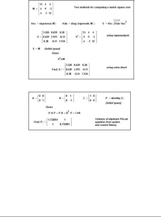
Example 4: A solve block for computing the square root of a matrix.
Example 5: A solve block for computing the solution of a matrix equation.
Comments Mathcad Professional lets you numerically solve a system of up to 200 simultaneous equations in 200 unknowns. (For Mathcad Standard, the upper limit is 50 equations in 50 unknowns.) If you aren’t sure that a given system possesses a solution but need an approximate answer which minimizes error, use Minerr instead. To solve an equation symbolically, that is, to find an exact numerical answer in terms of elementary functions, choose Solve for Variable from the Symbolic menu or use the solve keyword.
There are four steps to solving a system of simultaneous equations:
1.Provide initial guesses for all the unknowns you intend to solve for. These give Mathcad a place to start searching for solutions. Use complex guess values if you anticipate complex solutions; use real guess values if you anticipate real solutions.
2.Type the word Given. This tells Mathcad that what follows is a system of equality or inequality constraints. You can type Given or given in any style. Just don't type it while in a text region.
3.Type the equations and inequalities in any order below the word Given. Use [Ctrl]= to type “ =.”
34 |
Chapter 1 Functions |

4.Finally, type the Find function with your list of unknowns. You can’t put numerical values in the list of unknowns: for example, Find(2) in Example 1 isn’t permitted. Like given, you can type Find or find in any style.
The word Given, the equations and inequalities that follow, and the Find function form a solve block.
Example 1 shows a worksheet that contains a solve block for one equation in one unknown. For one equation in one unknown, you can also use the root or polyroots functions.
Mathcad is very specific about the types of expressions that can appear between Given and Find. See Example 2. The types of allowable constraints are z=w, x>y, x <y, x ³y and x £y. Mathcad does not allow the following inside a solve block:
•Constraints with “ ¹”
•Range variables or expressions involving range variables of any kind
•Inequalities of the form a < b < c
•Any kind of assignment statement (statements like x:=1)
If you want to include the outcome of a solve block in an iterative calculation, see Example 3.
Solve blocks cannot be nested inside each other. Each solve block can have only one Given and one Find. You can however, define a function like f(x) := Find(x ) at the end of one solve block and use this same function in another solve block.
If the solver cannot make any further improvements to the solution but the constraints are not all satisfied, then the solver stops and marks Find with an error message. This happens whenever the difference between successive approximations to the solution is greater than TOL and:
•The solver reaches a point where it cannot reduce the error any further.
•The solver reaches a point from which there is no preferred direction. Because of this, the solver has no basis on which to make further iterations.
•The solver reaches the limit of its accuracy. Roundoff errors make it unlikely that further computation would increase accuracy of the solution. This often happens if you set TOL to a value below 10– 15 .
The following problems may cause this sort of failure:
•There may actually be no solution.
•You may have given real guesses for an equation with no real solution. If the solution for a variable is complex, the solver will not find it unless the starting value for that variable is also complex.
•The solver may have become trapped in a local minimum for the error values. To find the actual solution, try using different starting values or add an inequality to keep Mathcad from being trapped in the local minimum.
•The solver may have become trapped on a point that is not a local minimum, but from which it cannot determine where to go next. Again, try changing the initial guesses or adding an inequality to avoid the undesirable stopping point.
•It may not be possible to solve the constraints to within the desired tolerance. Try defining TOL with a larger value somewhere above the solve block. Increasing the tolerance changes what Mathcad considers close enough to call a solution.
Functions |
35 |

Algorithm
See also
In Mathcad Professional, the context menu (available via right mouse click) associated with Find contains the following options:
•AutoSelect − chooses an appropriate algorithm
•Linear option − indicates that the problem is linear (and thus applies linear programming methods to the problem); guess values for var1, var2,... are immaterial (can all be zero)
•Nonlinear option − indicates that the problem is nonlinear (and thus applies these general
methods to the problem: the conjugate gradient solver; if that fails to converge, the Leven- berg-Marquadt solver; if that too fails, the quasi-Newton solver) − guess values for var1,
var2,... greatly affect the solution
•Quadratic option (appears only if the Mathcad Expert Solver product is installed) − indicates
that the problem is quadratic (and thus applies quadratic programming methods to the problem); guess values for var1, var2,... are immaterial (can all be zero)
•Advanced options − applies only to the nonlinear conjugate gradient and the quasi-Newton solvers
These options provide you more control in trying different algorithms for testing and comparison. You may also adjust the values of the built-in variables CTOL and TOL. The constraint tolerance CTOL controls how closely a constraint must be met for a solution to be acceptable; if CTOL were 0.001, then a constraint such as x < 2 would be considered satisfied if the value of x satisfied x < 2.001. This can be defined or changed in the same way as the convergence tolerance TOL. The default value for CTOL is 0.
For the non-linear case: Levenberg-Marquardt, Quasi-Newton, Conjugate Gradient For the linear case: simplex method with branch/bound techniques
(Press et al., 1992; Polak, 1997; Winston, 1994)
Minerr, Maximize, Minimize
floor |
Truncation and Round-off |
Syntax floor(x)
Description Returns the greatest integer ≤ x.
Arguments
x real number
Example
Comments Can be used to define the positive fractional part of a number: mantissa(x) := x - floor(x).
See also ceil, round, trunc
36 |
Chapter 1 Functions |

gcd |
Number Theory/Combinatorics |
Syntax gcd(A)
Description Returns the largest positive integer that is a divisor of all the values in the array A. This integer is known as the greatest common divisor of the elements in A.
Arguments
A integer matrix or vector; all elements of A are greater than zero
Algorithm Euclid’s algorithm (Niven and Zuckerman, 1972)
See also |
lcm |
genfit
Syntax
Description
Arguments
Regression and Smoothing
genfit(vx, vy, vg, F)
Returns a vector containing the parameters that make a function f of x and n parameters u0, u1, ¼, un – 1 best approximate the data in vx and vy.
vx, vy real vectors of the same size
vg real vector of guess values for the n parameters
Fa function that returns an n+1 element vector containing f and its partial derivatives with respect to its n parameters
Example
Functions |
37 |

Comments
Algorithm
See also
The functions linfit and genfit are closely related. Anything you can do with linfit you can also do, albeit less conveniently, with genfit. The difference between these two functions is analogous to the difference between solving a system of linear equations and solving a system of nonlinear equations. The former is easily done using the methods of linear algebra. The latter is far more difficult and generally must be solved by iteration. This explains why genfit needs a vector of guess values as an argument and linfit does not.
The example above uses genfit to find the exponent that best fits a set of data. By decreasing the value of the built-in TOL variable, higher accuracy in genfit might be achieved.
Levenberg-Marquardt (Press et al., 1992)
linfit
geninv
Syntax
Description
Arguments
A
Comments
Algorithm
(Professional) |
Vector and Matrix |
geninv(A)
Returns the left inverse of a matrix A.
real m ´ n matrix, where m ³ n .
If L denotes the left inverse, then L × A = I where I is the identity matrix with cols(I)=cols(A).
SVD-based construction (Nash, 1979)
genvals |
(Professional) |
Vector and Matrix |
Syntax genvals(M, N)
Description Returns a vector v of eigenvalues each of which satisfies the generalized eigenvalue equation M × x = vj × N × x for nonzero eigenvectors x.
Arguments
M, N real square matrices of the same size
38 |
Chapter 1 Functions |

Example
Comments To compute the eigenvectors, use genvec.
Algorithm Stable QZ method (Golub and Van Loan, 1989)
genvecs |
(Professional) |
Vector and Matrix |
Syntax genvecs(M, N)
Description Returns a matrix of normalized eigenvectors corresponding to the eigenvalues in v, the vector returned by genvals. The jth column of this matrix is the eigenvector x satisfying the generalized eigenvalue problem M × x = vj × N × x .
Arguments
M, N |
real square matrices of the same size |
|
|
|
Algorithm |
Stable QZ method (Golub and Van Loan, 1989) |
|
|
|
See also |
genvals for example |
|
|
|
|
|
|
|
|
gmean |
|
|
|
Statistics |
Syntax |
gmean(A) |
æm – 1 n – 1 |
ö 1 ¤ (mn) |
|
|
|
|||
Description |
Returns the geometric mean of the elements of A: gmean(A) |
= ç ∏ ∏ Ai, j÷ |
. |
|
Arguments |
|
è i = 0 j = 0 |
ø |
|
real m × n matrix or vector with all elements greater than zero |
|
|
|
|
A |
|
|
|
|
See also |
hmean, mean, median, mode |
|
|
|
Functions |
39 |

Her |
(Professional) |
Special |
Syntax |
Her(n, x) |
|
Description |
Returns the value of the Hermite polynomial of degree n at x. |
|
Arguments |
integer, n ³ 0 |
|
n |
|
|
x |
real number |
|
Comments The nth degree Hermite polynomial is a solution of the differential equation:
d2 |
d |
× n × y= 0 . |
|
x × -------y – |
2 × x × ----- y + 2 |
||
dx |
2 |
dx |
|
|
|
|
|
Algorithm Recurrence relation (Abramowitz and Stegun, 1972)
hist
Syntax
Description
Arguments
Statistics
hist(intervals, A)
Returns a vector containing the frequencies with which values in A fall in the intervals represented by the intervals vector. The resulting histogram vector is one element shorter than intervals.
intervals real vector with elements in ascending order
A real matrix
Example
40 |
Chapter 1 Functions |

Comments The intervals vector contains the endpoints of subintervals constituting a partition of the data. The result of the hist function is a vector f, in which fi is the number of values in A satisfying the condition intervalsi £ value < intervalsi + 1 .
Mathcad ignores data points less than the first value in intervals or greater than the last value in intervals.
hmean
Syntax
Description
Arguments
A
See also
|
|
|
|
|
|
|
|
Statistics |
hmean(A) |
|
|
æ |
|
|
|
|
ö – 1 |
|
|
|
1 |
m – 1 |
n – 1 |
|||
Returns the harmonic mean of the elements of A: |
hmean(A) |
|
ç |
|
å å |
1 ÷ |
||
= |
ç |
------ |
÷ |
|||||
|
|
|
--------- . |
|||||
èmn i = 0 j = 0 Ai, øj
real or complex m × n matrix or vector with all elements nonzero gmean, mean, median, mode
I0 |
|
Bessel |
Syntax |
I0(x) |
|
Description |
Returns the value of the modified Bessel function I0(x) |
of the first kind. Same as In(0, x). |
Arguments |
|
|
x |
real number |
|
Algorithm |
Small order approximation (Abramowitz and Stegun, 1972) |
|
|
|
|
I1 |
|
Bessel |
Syntax |
I1(x) |
|
Description |
Returns the value of the modified Bessel function I1(x) |
of the first kind. Same as In(1, x). |
Arguments |
|
|
x |
real number |
|
Algorithm |
Small order approximation (Abramowitz and Stegun, 1972) |
|
Functions |
41 |

ibeta
Syntax
Description
Arguments
a
x, y
Comments
Algorithm
(Professional) |
Special |
ibeta(a, x, y)
Returns the value of the incomplete beta function with parameter a, at (x, y).
real number, 0 £ a £ 1 real numbers, x > 0, y > 0
The incomplete beta function often arises in probabilistic applications. It is defined by the following formula:
ibeta(a, x, y ) = |
G(x + y ) |
a |
x – 1 |
× (1 – t) |
y – 1 |
dt . |
-------------------------- × |
t |
|
|
|||
|
G(x) × G(y) |
ò0 |
|
|
|
|
Continued fraction expansion (Abramowitz and Stegun, 1972)
icfft |
Fourier Transform |
Syntax icfft(A)
Description Returns the inverse Fourier transform corresponding to cfft. Returns an array of the same size as its argument.
Arguments
A real or complex matrix or vector
Comments |
The cfft and icfft functions are exact inverses; icfft(cfft(A)) = A . |
Algorithm Singleton method (Singleton, 1986)
See also fft for more details and cfft for example
ICFFT |
Fourier Transform |
Syntax ICFFT(A)
Description Returns the inverse Fourier transform corresponding to CFFT. Returns an array of the same size as its argument.
Arguments
A real or complex matrix or vector
Comments The CFFT and ICFFT functions are exact inverses; ICFFT(CFFT(A)) = A .
Algorithm Singleton method (Singleton, 1986)
See also fft for more details and CFFT for example
42 |
Chapter 1 Functions |