

funct_a_l
.pdfdgeom |
Probability Density |
Syntax |
dgeom(k, p) |
Description |
Returns Pr(X = k) when the random variable X has the geometric distribution: p(1 – p )k . |
Arguments |
|
k |
integer, k ³ 0 |
p |
real number, 0 < p £ 1 |
dhypergeom
Syntax
Description
Arguments
Probability Density
dhypergeom(m, a, b, n)
Returns Pr(X = m) when the random variable X has the hypergeometric distribution:
æ a ö |
× æ b ö |
¤ æa + bö |
where max{0, n – b} £ m £ min{n, a} ; 0 for m elsewhere. |
èmø |
èn – mø |
è n ø |
|
m, a, b, n integers, 0 £ m £ a , 0 £ n – m £ b , 0 ≤ n ≤ a + b
diag |
(Professional) |
|
|
Vector and Matrix |
||
Syntax |
diag(v) |
|
|
|
|
|
Description |
Returns a diagonal matrix containing, on its diagonal, the elements of v. |
|
|
|
||
Arguments |
|
|
|
|
|
|
v |
real or complex vector |
|
|
|
|
|
|
|
|
|
|||
dlnorm |
|
|
Probability Density |
|||
Syntax |
dlnorm(x, μ, σ) |
|
|
|
|
|
Description |
Returns the probability density for the lognormal distribution: ------------ |
1 ----- |
exp |
æ– |
--------1 ( ln (x) – |
m)2ö . |
Arguments |
2psx |
|
è |
2s2 |
ø |
|
|
|
|
|
|
|
|
x |
real number, x ³ 0 |
|
|
|
|
|
μ |
real logmean |
|
|
|
|
|
σ |
real logdeviation, σ > 0 |
|
|
|
|
|
Functions |
23 |

dlogis |
|
Probability Density |
Syntax |
dlogis(x, l, s) |
|
Description |
|
exp (– (x – l) ¤ s) |
Returns the probability density for the logistic distribution: |
s----------------------------------------------------------(1 + exp (– (x – l ) ¤ s))2 . |
|
Arguments |
|
|
x |
real number |
|
l |
real location parameter |
|
s |
real scale parameter, s > 0 |
|
dnbinom |
|
|
|
Probability Density |
Syntax |
dnbinom(k, n, p) |
|
||
Description |
Returns Pr(X = k) when the random variable X has the negative binomial distribution: |
|||
|
æn + k – 1ö pn(1 – |
p)k |
||
|
è |
k |
ø |
|
|
|
|
|
|
Arguments
k, n integers, n > 0 and k ³ 0 p real number, 0 < p £ 1
dnorm |
|
|
Probability Density |
|
Syntax |
dnorm(x, μ, s) |
|
|
|
Description |
1 |
æ |
1 |
m)2ö . |
Returns the probability density for the normal distribution: -------------- exp |
– --------(x – |
|||
|
2ps |
è |
2s2 |
ø |
Arguments
xreal number
μreal mean
σreal standard deviation, σ > 0
Example
24 |
Chapter 1 Functions |

dpois
Syntax
Description
Arguments
Probability Density
dpois(k, λ)
Returns Pr( X = k) when the random variable X has the Poisson distribution: lk e– l .
-----
k!
k integer, k ³ 0
λ real mean, l > 0
dt |
Probability Density |
|||
Syntax |
dt(x, d) |
|
|
|
Description |
G((d + 1) ¤ 2 )æ |
x2ö |
– (d + 1) ¤ 2 |
|
Returns the probability density for Student’s t distribution: -------------------------------- |
è |
1 + ---- |
. |
|
Arguments |
G(d ¤ 2) pd |
d ø |
|
|
|
|
|
|
|
x |
real number |
|
|
|
d |
integer degrees of freedom, d > 0 |
|
|
|
dunif |
Probability Density |
Syntax |
dunif(x, a, b) |
Description |
1 |
Returns the probability density for the uniform distribution: ----------- . |
|
|
b – a |
Arguments |
|
x |
real number, a £ x £ b |
a, b |
real numbers, a < b |
dweibull |
Probability Density |
Syntax |
dweibull(x, s) |
Description |
Returns the probability density for the Weibull distribution: sxs – 1 exp (– xs ) . |
Arguments |
|
x |
real number, x ³ 0 |
s |
real shape parameter, s > 0 |
eigenvals |
Vector and Matrix |
Syntax |
eigenvals(M) |
Description |
Returns a vector of eigenvalues for the matrix M. |
Arguments |
|
M |
real or complex square matrix |
Functions |
25 |

Example
Algorithm Reduction to Hessenberg form coupled with QR decomposition (Press et al., 1992)
See also eigenvec, eigenvecs
eigenvec
Syntax
Description
Arguments
Vector and Matrix
eigenvec(M, z)
Returns a vector containing the normalized eigenvector corresponding to the eigenvalue z of the square matrix M.
M real or complex square matrix
z real or complex number
Algorithm Inverse iteration (Press et al., 1992; Lorczak)
See also eigenvals, eigenvecs
eigenvecs
Syntax
Description
Arguments
(Professional) |
Vector and Matrix |
eigenvecs(M)
Returns a matrix containing the normalized eigenvectors corresponding to the eigenvalues of the matrix M. The nth column of the matrix is the eigenvector corresponding to the nth eigenvalue returned by eigenvals.
M real or complex square matrix
Algorithm Reduction to Hessenberg form coupled with QR decomposition (Press et al., 1992)
See also eigenvals, eigenvec
26 |
Chapter 1 Functions |

Example
erf
Syntax
Description
Arguments
x
Algorithm
See also
Special
erf(x)
Returns the error function erf (x ) |
|
x |
2 |
2 |
|
= |
ò0 |
π |
|
dt . |
|
|
------e– t |
|
real number
Continued fraction expansion (Abramowitz and Stegun, 1972; Lorczak)
erfc
erfc |
Special |
Syntax |
erfc(x) |
Description |
Returns the complementary error function erfc(x ) := 1 – erf(x) . |
Arguments |
|
x |
real number |
Algorithm |
Continued fraction expansion (Abramowitz and Stegun, 1972; Lorczak) |
See also |
erf |
Functions |
27 |

error
Syntax
Description
Arguments
S
Example
Comments
(Professional) |
String |
error(S)
Returns the string S as an error message.
string
Mathcad’s built-in error messages appear as “error tips” when a built-in function is used incorrectly or could not return a result.
Use the string function error to define specialized error messages that will appear when your user-defined functions are used improperly or cannot return answers.This function is especially useful for trapping erroneous inputs to Mathcad programs you write.
When Mathcad encounters the error function in an expression, it highlights the expression in red. When you click on the expression, the error message appears in a tool tip that hovers over the expression. The text of the message is the string argument you supply to the error function.
exp |
Log and Exponential |
Syntax |
exp(z) |
Description |
Returns the value of the exponential function ez . |
Arguments |
|
z |
real or complex number |
fft |
Fourier Transform |
Syntax |
fft(v) |
Description |
Returns the fast discrete Fourier transform of real data. Returns a vector of size 2n – 1 + 1 . |
Arguments |
|
v |
real vector with 2n elements (representing measurements at regular intervals in the time |
|
domain), where n is an integer, n > 0. |
28 |
Chapter 1 Functions |
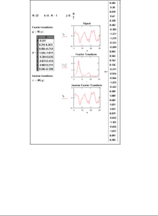
Example
Comments When you define a vector v for use with Fourier or wavelet transforms, be sure to start with v0 (or change the value of ORIGIN). If you do not define v0 , Mathcad automatically sets it to zero. This can distort the results of the transform functions.
Mathcad comes with two types of Fourier transform pairs: fft/ifft and cfft/icfft . These functions can be applied only to discrete data (i.e., the inputs and outputs are vectors and matrices only). You cannot apply them to continuous data.
Use the fft and ifft functions if:
•the data values in the time domain are real, and
•the data vector has 2m elements.
Use the cfft and icfft functions in all other cases.
Functions |
29 |

The first condition is required because the fft/ifft pair takes advantage of the fact that, for real data, the second half of the transform is just the conjugate of the first. Mathcad discards the second half of the result vector to save time and memory. The cfft/icfft pair does not assume symmetry in the transform; therefore you must use this pair for complex valued data. Because the real numbers are just a subset of the complex numbers, you can use the cfft/icfft pair for real numbers as well.
The second condition is required because the fft/ifft transform pair uses a highly efficient fast Fourier transform algorithm. In order to do so, the vector you use with fft must have 2m elements. The cfft/icfft Fourier transform pair uses an algorithm that permits vectors as well as matrices of arbitrary size. When you use this transform pair with a matrix, you get back a two-dimensional Fourier transform.
If you used fft to get to the frequency domain, you must use ifft to get back to the time domain. Similarly, if you used cfft to get to the frequency domain, you must use icfft to get back to the time domain.
Different sources use different conventions concerning the initial factor of the Fourier transform and whether to conjugate the results of either the transform or the inverse transform. The functions fft, ifft, cfft, and icfft use 1 ¤ N as a normalizing factor and a positive exponent in going from the time to the frequency domain. The functions FFT, IFFT, CFFT, and ICFFT use 1 ¤ N as a normalizing factor and a negative exponent in going from the time to the frequency domain. Be sure to use these functions in pairs. For example, if you used CFFT to go from the time domain to the frequency domain, you must use ICFFT to transform back to the time domain.
The elements of the vector returned by fft satisfy the following equation:
|
1 |
n – 1 |
cj |
|
|
= ------ å vke2pi (j ¤ n)k |
||
|
n |
k = 0 |
|
|
|
In this formula, n is the number of elements in v and i is the imaginary unit.
The elements in the vector returned by the fft function correspond to different frequencies. To recover the actual frequency, you must know the sampling frequency of the original signal. If v is an n-element vector passed to the fft function, and the sampling frequency is fs , the frequency corresponding to ck is
fk |
k |
× fs |
= -- |
||
|
n |
|
Therefore, it is impossible to detect frequencies above the sampling frequency. This is a limitation not of Mathcad, but of the underlying mathematics itself. In order to correctly recover a signal from the Fourier transform of its samples, you must sample the signal with a frequency of at least twice its bandwidth. A thorough discussion of this phenomenon is outside the scope of this manual but within that of any textbook on digital signal processing.
Algorithm Cooley-Tukey (Press et al., 1992)
30 |
Chapter 1 Functions |

FFT |
Fourier Transform |
Syntax |
FFT(v) |
Description |
Identical to fft(v), except uses a different normalizing factor and sign convention. Returns a vector |
|
of size 2n – 1 + 1 . |
Arguments
vreal vector with 2n elements (representing measurements at regular intervals in the time domain), where n is an integer, n > 0.
Comments |
The definitions for the Fourier transform discussed in the fft entry are not the only ones used. |
|
|
For example, the following definitions for the discrete Fourier transform and its inverse appear |
|
|
in Ronald Bracewell’s The Fourier Transform and Its Applications (McGraw-Hill, 1986): |
|
|
n |
n |
|
1 |
å F(υ)e2pi(t ¤ n)u |
|
F(υ) = n-- å f(τ )e– 2pi(u ¤ n)t f(τ) = |
|
|
t = 1 |
u = 1 |
|
These definitions are very common in engineering literature. To use these definitions rather than |
|
|
those presented in the last section, use the functions FFT, IFFT, CFFT, and ICFFT. These differ |
|
|
from those discussed in the last section as follows: |
|
|
• Instead of a factor of 1/ n in front of both forms, there is a factor of 1/n in front of the |
|
|
transform and no factor in front of the inverse. |
|
|
• The minus sign appears in the exponent of the transform instead of in its inverse. |
|
|
The functions FFT, IFFT, CFFT, and ICFFT are used in exactly the same way as the functions |
|
|
fft, ifft, cfft, and icfft. |
|
Algorithm |
Cooley-Tukey (Press et al., 1992) |
|
See also |
fft for more details |
|
|
|
|
fhyper |
(Professional) |
Special |
Syntax |
fhyper(a, b, c, x) |
|
Description |
Returns the value of the Gauss hypergeometric function 2F1(a, b;c;x ) . |
|
Arguments |
real numbers, – 1 < x < 1 |
|
a, b, c, x |
|
|
Functions |
31 |

Comments
Algorithm
The hypergeometric function is a solution of the differential equation
x × (1 – |
d2 |
d |
|
x ) × -------y + (c – |
(a + b + 1) × x ) × -----y – a × b × y= 0 . |
||
|
dx |
2 |
dx |
|
|
|
|
Many functions are special cases of the hypergeometric function, e.g., elementary ones like
ln (1 + x) = x × fhyper(1, 1, 2, – x) , |
asin (x) = x × fhyper |
1 |
1 |
3 |
2 |
, |
æ--, --, --, x |
ö |
|||||
|
|
è2 |
2 |
2 |
ø |
|
and more complicated ones like Legendre functions.
Series expansion (Abramowitz and Stegun, 1972)
Find |
Solving |
Syntax Find(var1, var2, ...)
Description Returns values of var1, var2, ... which solve a prescribed system of equations, subject to prescribed inequalities. The number of arguments matches the number of unknowns. Output is a scalar if only one argument; otherwise it is a vector of answers.
Arguments
var1, var2, ... real or complex variables; var1, var2,.. must be assigned guess values before using Find.
Examples
Example 1: A solve block with one equation in one unknown.
32 |
Chapter 1 Functions |