

09.Robustness and performance
.pdf9.10. SPECIFICATIONS |
263 |
²Maximum complementary sensitivity Mt.
²Frequency where the complementary sensitivity function has its maximum !ms.
Another set of speci¯cations is based on a Taylor series expansion of the transfer function Ged(s) from a disturbance to the error
Ged(s) = e0 + e1s + e2s2 + ¢¢¢ :
The numbers ei are called error coe±cients. The ¯rst coe±cient that is not zero is of particular interest. Assume for example that the ¯rst nonvanishing error coe±cient is e2. It means that constant disturbance and linearly increasing disturbances do not give any steady state errors and that the jerk disturbance d(t) = kt2 gives a constant steady state error ke2.
Relations between Time and Frequency Domain Features
There are approximate relations between speci¯cations in the time and frequency domain. Let G(s) be the transfer function from setpoint to output. In the time domain the response speed can be characterized by the rise time Tr , the average residence time Tar or the settling time Ts. In the frequency domain the response time can be characterized by the closed loop bandwidth !b, the gain crossover frequency !gc, the sensitivity frequency !ms. The product of bandwidth and rise time is approximately constant Tr !b ¼ 2. The overshoot of the step response o is related to the peak Mp of the frequency response in the sense that a larger peak normally implies a lager oveshoot. Unfortunately there are no simple relation because the overshoot also depends on how quickly the frequency response decays. For Mp < 1:2 the overshoot o in the step response is often close to Mp ¡ 1. For larger values of Mp the overshoot is typically less than Mp ¡ 1. These relations do not hold for all systems, there are systems with Mp = 1 that have a positive overshoot. These systems have a transfer functions that decay rapidly around the bandwidth. To avoid overshoots in systems with error feedback it is advisable to require that the maximum of the complementary sensitivity function is small, say Mt = 1:1 ¡ 1:2.
Response to Load Disturbances
The sensitivity function (9.20) shows how feedback in°uences disturbances. Disturbances with frequencies that are lower than the sensitivity crossover
264 CHAPTER 9. ROBUSTNESS AND PERFORMANCE
frequency !sc are attenuated by feedback and those with ! > !sc are ampli¯ed by feedback. The largest ampli¯cation is the maximum sensitivity
Ms.
Consider the system in Figure 9.2. The transfer function from load
disturbance d to process variable is |
|
|
|
|
|
Gxd = |
P |
= P S = |
T |
: |
(9.33) |
|
|
||||
1 + P C |
C |
||||
Since load disturbances typically have low frequencies it is natural that the criterion emphasizes the behavior of the transfer function at low frequencies. Filtering of the measurement signal has only marginal e®ect on the attenuation of load disturbances because the ¯lter only attenuates high frequencies. For a system with P (0) =6 0 and a controller with integral action control the controller gain goes to in¯nity for small frequencies and we have the following approximation for small s
Gxd = |
T |
1 |
|
s |
|
|
|
|
¼ |
|
¼ |
|
: |
(9.34) |
|
C |
C |
ki |
|||||
Since load disturbances typically have low frequencies the integral gain ki is a good measure of load disturbance rejection for systems where the controller has integral action. Figure 9.22 which gives the gain curve for a typical case shows that the approximation is very good for low frequencies. transfer functions. Measurement noise, which typically has high frequencies, generates rapid variations in the control variable which are detrimental because they cause wear in valves and motors and they can even saturate the actuator. It is important to keep the variations in the control signal at reasonable levels. A typical requirement is that the variations are only a fraction of the span of the control signal. The variations can be in°uenced by ¯ltering and by proper design of the high frequency properties of the controller.
The e®ects of measurement noise are captured by the transfer function from measurement noise to the control signal
Gun = |
C |
= CS = |
T |
: |
(9.35) |
|
|
||||
1 + P C |
P |
Figure 9.22 shows the gain curve of Gun for a typical system. For low frequencies the transfer function the sensitivity function equals 1 and (9.35) can be approximated by 1=P (s). For high frequencies is is approximated as
Gun ¼ C(s).
9.10. SPECIFICATIONS |
265 |
j |
100 |
|
|
|
|
|
|
(!) |
|
|
|
|
|
|
|
xd |
|
|
|
|
|
|
|
G |
−2 |
|
|
|
|
|
|
j |
|
|
|
|
|
|
|
10 |
|
|
|
|
|
|
|
|
|
|
|
|
|
|
|
|
10−3 |
10−2 |
10−1 |
100 |
101 |
102 |
103 |
(!)j |
101 |
|
|
|
|
|
|
|
|
|
|
|
|
|
|
un |
100 |
|
|
|
|
|
|
jG |
|
|
|
|
|
|
|
|
10−3 |
10−2 |
10−1 |
100 |
101 |
102 |
103 |
|
|
|
|
! |
|
|
|
Figure 9.22: Gains of the transfer functions Gxd and Gun for PID control (k = 2:235, Ti = 3:02, Ti = 0:756 and Tf = T d=5) of the process P = (s + 1)¡4. The the gain of the transfer functions P (s), C(s), 1=C(s) are shown with dashed lines and s=ki with dash-dotted lines.
A simple measure of the e®ect of measurement noise is the high frequency gain of the transfer function Gun
Mun = |
max |
G |
|
(i!) |
: |
(9.36) |
! j |
|
un |
j |
|
|
A more accurate measure is the standard deviation of the control signal. If the power spectrum of measurement noise is 'n(!), the standard deviation of the control signal is
1 |
|
¾u2 = Z¡1 jGun(i!)j2Án(!)d!: |
(9.37) |
Tradeo®s
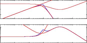
There are many tradeo®s in control design, one is between load disturbance rejection and measurement noise injection. This is illustrated in Figure 9.23 where a process with the transfer function P (s) = 1=(s + 1)4 is controlled with PI (k = 0:5 and Ti = 2) and PID (k = 2:235, Ti = 3:02, Ti = 0:756 and Tf = T d=5) controllers. The ¯gure shows that the PID controller gives better attenuation of load disturbances k=0:74 as compared with ki = 0:25 for PI control. This is also illustrated in the time responses for load disturbances where the maximum error is much smaller emax = 0:38 for PID control and

266 |
CHAPTER 9. ROBUSTNESS AND PERFORMANCE |
jGxd (!)j
100
10−1
10−2
exd
10−2 |
100 |
102 |
0.6 |
|
|
|
|
|
0.4 |
|
|
|
|
|
0.2 |
|
|
|
|
|
0 |
|
|
|
|
|
−0.2 |
5 |
10 |
15 |
20 |
25 |
0 |
(!)j |
101 |
|
|
||
un |
100 |
|
jG |
||
|
|
|
|
1.5 |
|
|
|
|
|
|
|
|
1 |
|
|
|
|
|
|
|
|
xd |
|
|
|
|
|
|
|
|
u |
|
|
|
|
|
|
|
|
0.5 |
|
|
|
|
|
10−2 |
100 |
102 |
00 |
5 |
10 |
15 |
20 |
25 |
|
! |
, |
|
|
|
t |
|
|
Figure 9.23: Illustrates trade o® between attenuation of load disturbances and measurement noise injection. The ¯gure on the left shows the gain curves of the transfer functions Gxd(s) and Gun(s) and the curves on the right shows the time responses to steps in the load disturbance. Results for PID control are shown in full lines and for PI with dashed lines.
emax = 0:69 for PI control. Analyzing the control signals we ¯nd that the bene¯t by PID control is primarily due to the fact that the controller reacts faster to the disturbance. The penalty for the improved performance is that the largest gain of the transfer function Gun is Mun = 11:2 for PID control as compared to Mun = 1:2 for PI control.
Summary
Summarizing we ¯nd that the behavior of a closed loop system system can be characterized by the following four parameters:
²Load disturbance attenuation is described by integral gain ki
²Measurement noise injection is described by the high frequency gain Mun of the transfer function from measurement noise to control signal.
²Robustness to process variations is described by the maximum sensitivities Ms and Mt
9.11. FURTHER READING |
267 |
For systems permitting a controller with two degrees of freedom the desired response to command signal can be adjusted by feedforward. For systems with error feedback the overshoot of the response to load disturbances can be speci¯ed by Mt.
9.11Further Reading
Bodes book, classical control, Doyle Francis Tannenbaum, Zhou and Doyle Vinnicombe.
9.12Exercises
268 |
CHAPTER 9. ROBUSTNESS AND PERFORMANCE |