

09.Robustness and performance
.pdf9.8. IMPLICATIONS FOR DESIGN |
253 |
Design Rules
Let the transfer functions of the process and the controller be
P (s) = np(s) dp(s)
C(s) = nc(s) dc(s)
where np(s), nc(s), dp(s) and dc(s) are polynomials. The sensitivity functions then becomes
S(s) = |
dp(s)dc(s) |
dp(s)dc(s) + np(s)dp(s) |
|
T (s) = |
np(s)nc(s) |
dp(s)dc(s) + np(s)dp(s) |
Let wgc be the desired gain crossover frequency. Assume that the process has zeros which are slower than !gc. The complementary sensitivity function is one for low frequencies and it start to increase for frequencies close to the process zeros unless there is a closed loop pole in the neighborhood. To avoid large values of the complementary sensitivity function we ¯nd that the closed loop system should have poles close to the slow zeros.
Now consider process poles that are faster than the desired gain crossover frequency. The sensitivity function is one for high frequencies. Moving from high to low frequencies the sensitivity function increases at the fast process poles. Large peaks can be obtained unless there are process poles close to the closed loop poles. To avoid large peaks in the sensitivity the closed loop system should be have poles close that matches the fast process poles. We thus obtain the simple rules that slow process zeros should be matched slow closed loop poles and fast process poles should be matched by fast process poles. The rule are illustrated with an additional example.
Example 9.4 (To Cancel or not to Cancel). Consider PI control of a ¯rst order system where the process and the controller have the transfer functions
b P (s) = s + a
C(s) = k + ksi
The loop transfer function is
L(s) = b(ks + ki)
s(s + a)
254 |
CHAPTER 9. ROBUSTNESS AND PERFORMANCE |
jT (i!)j
100
10−2
10−4
10−2 |
100 |
102 |
|
! |
, |
jT (i!)j
100
10−2
10−4 |
|
|
10−2 |
100 |
102 |
!
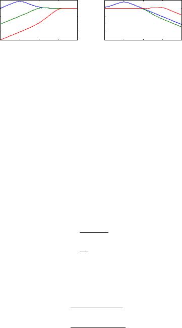
Figure 9.17: Magnitude curve for Bode plots of the sensitivity function S (above) and the complementary sensitivity function T (below) for ³ = 0:7, a = 1 and !0=a = 0:1 (dashed), 1 (solid) and 10 (dotted).
The closed loop characteristic polynomial is
s(s + a) + b(ks + ki) = s62 + (a + bk)s + ki
Let the desired closed loop characteristic polynomial be
s2 + 2³!0s + !02 |
(9.23) |
Matching this with we ¯nd that the controller gains are
s2 + 2³!0s + !02 |
(9.24) |
where ³ · 1, we ¯nd that the controller parameters are given by
k = 2³!0 ¡ a b
!2 ki = 0 b
Notice that the controller has a zero in the right half plane if 2³!0 < a, an indication that the system has bad properties. The sensitivity functions we get
S(s) =
s(s + a)
s2 + 2³!0s + !02
(2³!0 ¡ a)s + !2
T (s) = 0 s2 + 2³!0s + !02
Figure 9.17 shows clearly that the sensitivities are small for designs with !0 > a, but high for designs with !0 > a. If we desire a system with slower

9.9When are Two Processes Similar?
A fundamental issue is to determine when two processes are close. This seemingly innocent problem is not as simple as it may appear. When discussing the e®ects of uncertainty of the process on stability in Section 9.6 we used the quantity
±(P1; P2) = |
max |
P |
(i!) |
¡ |
P |
(i!) |
j |
(9.25) |
! j |
1 |
|
2 |
|
|
as a measure of closeness of two processes. In addition the transfer functions P1 and P2 were assumed to be stable. This means conceptually that we compare the outputs of two systems subject to the same input. This may appear as a natural way to compare two systems but there are complications. Two systems that have similar open loop behaviors may have drastically di®erent behavior in closed loop and systems with very di®erent open loop behavior may have similar closed loop behavior. We illustrate this by two examples.
256 |
CHAPTER 9. ROBUSTNESS AND PERFORMANCE |
|
100 |
|
|
|
|
)j |
102 |
|
|
|
|
|
|
|
100 |
||
|
|
|
|
|
|
(i! |
||
|
|
|
|
|
|
|
||
|
|
|
|
|
|
2 |
−2 |
|
|
|
|
|
|
|
1; |
||
|
|
|
|
|
|
10 |
||
|
|
|
|
|
|
jP |
||
|
|
|
|
|
|
|
||
y |
50 |
|
|
|
|
|
|
10−4 |
|
|
|
|
|
|
|
||
|
|
|
|
|
|
|
|
|
|
|
|
|
|
|
(i!) |
|
0 |
|
|
|
|
|
|
|
−90 |
|
|
|
|
|
|
|
1;2 |
|
|
|
|
|
|
|
|
|
|
|
|
|
|
|
|
|
P |
−180 |
|
|
|
|
|
|
|
arg |
||
|
0 |
|
|
|
|
−270 |
||
|
0 |
2 |
4 |
6 |
8 |
|
||
|
|
|
|
|||||
|
|
|
t |
|
|
|
|
|
10−2 |
100 |
102 |
10−2 |
100 |
102 |
!
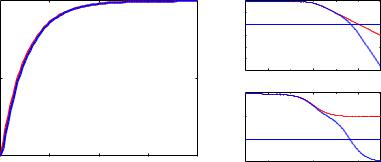
Figure 9.18: Step responses for systems with the transfer functions P1(s) = 100=(s + 1) (dashed) and P2(s) = 160000=((s + 1)(s + 40)2) (full).
Example 9.5 (Similar in Open Loop but Di®erent in Closed Loop). Systems with the transfer functions
100 |
|
|
100a2 |
|
P1(s) = |
|
; |
P2(s) = |
|
s + 1 |
(s + 1)(s + a)2 |
|||
have very similar open loop responses for large values of a. This is illustrated in Figure 9.18 which shows the step responses of for a = 40. The di®erences between the step responses are barely noticeable in the ¯gure. The transfer functions from reference values to output for closed loop systems obtained with error feedback with C = 1 are
100 |
|
|
161600 |
|
T1 = |
|
; |
T2 = |
|
s + 101 |
(s + 83:92)(s2 ¡ 2:9254s + 1925:5) |
|||
The closed loop systems are very di®erent because the system T1 is stable and T2 is unstable. Notice in Figure 9.18 that the Bode plots are very close for low frequencies but di®erent at high frequencies.
Example 9.6 (Di®erent in Open Loop but Similar in Closed Loop). Systems with the transfer functions
100 |
|
100 |
|
||
P1(s) = |
|
; |
P2(s) = |
|
|
s + 1 |
s ¡ 1 |
||||
have very di®erent open loop properties because one system is unstable and the other is stable. The transfer functions from reference values to output

9.9. WHEN ARE TWO PROCESSES SIMILAR? |
257 |
||||
for closed loop systems obtained with error feedback with C = 1 are |
|
||||
100 |
100 |
|
|
||
T1(s) = |
|
T2(s) = |
|
|
|
s + 101 |
s + 99 |
|
|||
which are very close.
These examples show clearly that to compare two systems by investigating their open loop properties may be strongly misleading from the point of view of feedback control. Inspired by the examples we will instead compare the properties of the closed loop systems obtained when two processes P1 and P2 are controlled by the same controller C. To do this it will be assumed that the closed loop systems obtained are stable. The di®erence between the closed loop transfer functions is
±(P |
; P |
) = |
¯ |
P1C |
¡ |
|
P2C |
¯ |
= |
¯ |
(P1 ¡ P2)C |
¯ |
(9.26) |
|
1 + P1C |
1 + P2C |
(1 + P1C)(1 + P2C) |
||||||||||||
1 |
2 |
|
|
|
||||||||||
|
|
|
¯ |
|
|
|
|
¯ |
|
¯ |
|
¯ |
|
|
|
|
|
¯ |
|
|
|
|
¯ |
|
¯ |
|
¯ |
|
|
This is a natural way to express the closeness of the systems P1 and P2, when they are controlled by C. It can be veri¯ed that ± is a proper norm in the mathematical sense. There is one di±culty from a practical point of view because the norm depends on the feedback C. The norm has some interesting properties.
Assume that the controller C has high gain at low frequencies. For low
frequencies we have
±(P1; P2) ¼ P1 ¡ P2 P1P2C
If C is large it means that ± can be small even if the di®erence P1 ¡ P2 is large. For frequencies where the maximum sensitivity is large we have
±(P1; P2) ¼ Ms1Ms2jC(P1 ¡ P2)j
For frequencies where P1 and P2 have small gains, typically for high frequencies, we have
±(P1; P2) ¼ jC(P1 ¡ P2)j
This equation shows clearly the disadvantage of having controllers with large gain at high frequencies. The sensitivity to modeling error for high frequencies can thus be reduced substantially by a controller whose gain goes to zero rapidly for high frequencies. This has been known empirically for a long time and it is called high frequency roll o®.
258 |
CHAPTER 9. ROBUSTNESS AND PERFORMANCE |
9.10Speci¯cations
Having understood the fundamental properties of the basic feedback loop we will now quantify the requirements on a typical control system. Control problems are rich and there are many factors that have to be taken into account.
²Load disturbance attenuation
²Measurement noise response
²Robustness to process uncertainties
²Response to command signals
The emphasis on the di®erent factors depend on the particular problem. Robustness is important for all applications. Command signal following is the major issue in motion control, where it is desired that the system follows commanded trajectories. . This is called the servo problem. The typical process control problem is to keep the process variable close to the reference signal, which is changed only when production is altered. This is called the r egulation problem. Attenuation of load disturbances is therefore the key issue in process control. There are also situations where the purpose of control is not to keep the process variables at speci¯ed values. Control bu®ers is a typical example. The reason for using bu®ers is to smooth °ow variations. A good strategy is to apply control only when there is a risk that bu®ers tend to be empty or full.
An advantage with a structure having two degrees of freedom, or setpoint weighting, is that the problem of setpoint response can be decoupled from the response to load disturbances and measurement noise. The design procedure can then be divided into two independent steps.
²First design the feedback controller C that reduces the e®ects of load disturbances and the sensitivity to process variations without introducing too much measurement noise into the system.
²Then design the feedforward F to give the desired response to setpoints.
We will now discuss how speci¯cations can be expressed in terms properties of the transfer functions (9.12).
The linear behavior of the system is completely determined by six transfer functions (9.11), the Gang of Six. Neglecting setpoint response it is
9.10. SPECIFICATIONS |
259 |
e |
|
emax |
|
Tmax |
t |
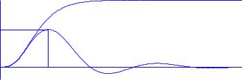
Figure 9.19: The error due to a unit step load disturbance some features used to characterize attenuation of load disturbances. The dashed curve show the open-loop error. The process transfer is P (s) = (s + 1)¡4 is controlled by a PI controller having parameters k = 1 and ki = 0:4 function is
su±cient to consider four transfer functions (9.12), the Gang of Four. Spec- i¯cations can be expressed in terms of these transfer functions. It is common practice to characterize the transfer functions by a few features.
Features of Time Responses
Many criteria are related to time responses, for example the step response to setpoint changes or the step response to load disturbances. It is common to use some feature of the error typically extrema, asymptotes, areas etc. The maximum error em is de¯ned as
emax = |
|
max |
j |
e(t) |
j |
||
0 |
· |
t< |
1 |
|
|||
|
|
|
|
|
(9.27) |
||
Tmax = arg max je(t)j:
The time Tmax where the maximum occurs is a measure of the response time of the system. An example is given in Figure 9.19 which shows the output for a step in the load disturbance. The closed loop system has !ms = 0:559, emax = 0:59 and Tmax = 5:15.
Other criteria are the integrated absolute error (IAE) |
|
|
IAE = Z0 |
1 je(t)jdt |
(9.28) |
the integrated error (IE) |
|
|
IE = Z 1 e(t)dt: |
(9.29) |
|
0
260 |
CHAPTER 9. ROBUSTNESS AND PERFORMANCE |
The criteria IE and IAE are the same if the error does not change sign. Notice that IE can be very small even if the error is not. For IE to be relevant it is necessary to add conditions that ensure that the error is not too oscillatory. The criterion IE is a natural choice for control of quality variables for a process where the product is sent to a mixing tank. The criterion may be strongly misleading, however, in other situations. It will be zero for an oscillatory system with no damping.
There are many other criteria, for example the time multiplied absolute error de¯ned by
Z 1
IT N AE = tnje(t)jdt: (9.30)
0
The integrated squared error (ISE) is de¯ned as
Z 1
ISE = e(t)2dt: (9.31)
0
There are other criteria that take account of both input and output signals for example the quadratic criterion
Z 1
QE = (e2(t) + ½u2(t))dt: (9.32)
0
where ½ is a weighting factor. The criteria IE and QE can easily be computed analytically, simulations are however required to determine IAE.
Response to Command Signals
Classical speci¯cations were strongly focused on the response of the output to step changes in the command signal. Many speci¯cations were developed for that response, for example rise time, settling time, decay ratio, overshoot, and steady-state o®set for step changes in setpoint. These quantities are de¯ned as follows, see Figure 9.20.
²The rise time Tr is de¯ned either as the inverse of the largest slope of the step response or the time it takes for the step response to change from 10% to 90% of its steady state value.
²The settling time Ts is the time it takes before the step response remains within p percent of its steady state value. The values p = 1; 2 and 5 percent of the steady state value are commonly used.
9.10. SPECIFICATIONS |
261 |
ysp |
o |
|
|
|
|
y0 |
|
2p% |
|
Tmax |
Ts |
umax |
u0 |
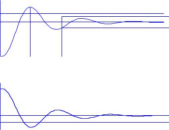
Figure 9.20: Speci¯cations on command signal following based on the time response to a unit step in the setpoint. The upper curve shows the response of the output and the lower curve shows the corresponding control signal.
²The decay ratio d is the ratio between two consecutive maxima of the error for a step change in setpoint or load. The value d = 1=4, which is called quarter amplitude damping, has been used traditionally. This value is, however, normally too high as will be shown later.
²The overshoot o is the ratio between the di®erence between the ¯rst peak and the steady state value and the steady state value of the step response. It is often given in%. In industrial control applications it is common to specify an overshoot of 8%{10%. In many situations it is desirable, however, to have an over-damped response with no overshoot.
²The steady-state error ess = ysp ¡ y0 is the steady state control error e. This is always zero for a controller with integral action.
Actuators may have rate limitations which means that step changes in the control signal will not appear instantaneously. In motion control systems it is often more relevant to consider responses to ramp signals instead of step signals.
262 |
CHAPTER 9. ROBUSTNESS AND PERFORMANCE |
Mp |
|
1 |
|
1=p2 |
|
!p |
!b |
Figure 9.21: Gain curve for transfer function from setpoint to output.
Features of Frequency Responses
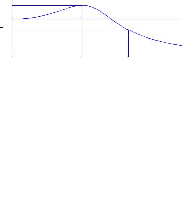
Speci¯cations can also be related to frequency responses. Since speci¯cations were originally focused on setpoint response it was natural to consider the transfer function from setpoint to output. A typical gain curve for this response is shown in Figure 9.21. It is natural to require that the steady state gain is one. Typical speci¯cations are then.
²The resonance peak Mp is the largest value of the frequency response.
²The peak frequency !p is the frequency where the maximum occurs.
²The bandwidth !b is the frequency where the gain has decreased to p
1= 2.
For a system with error feedback the transfer function from setpoint to output is equal to the complementary transfer function and we have Mp =
Mt.
Speci¯cations can also be related to the loop transfer function. Useful features that have been discussed previously are:
²Gain crossover frequency !gc.
²Gain margin gm.
²Phase margin 'm.
²Maximum sensitivity Ms.
²Frequency where the sensitivity function has its maximum !ms.
²Sensitivity crossover frequency !sc.