


page 10
2.1.4 Polynomial Expansions
• Binomial expansion for polynomials,
(a + x ) = a |
n |
+ na |
n – 1 |
x + n-------------------(n – 1 )a |
n – 2 |
x |
2 |
+ … + x |
n |
n |
|
|
|
|
|||||
|
|
|
|
2! |
|
|
|
|
|
2.2 FUNCTIONS
2.2.1 Discrete and Continuous Probability Distributions
• The Binomial distribution is,
P(m ) = ∑ |
n |
t |
|
n – t |
q = 1 – p |
q,p [0,1 ] |
|
t p |
q |
|
|
||||
t ≤ m |
|
|
|
|
|
|
|
• The Poisson distribution is, |
|
|
|
|
|
|
|
|
λ |
te–λ |
|
λ >0 |
|
||
P(m ) = ∑ ------------ |
|
||||||
t ≤ m |
t! |
|
|
|
|
||
|
|
|
|
|
|
||
• The Hypergeometric distribution is, |
|
|
|||||
|
r |
s |
|
|
|
||
P(m ) = ∑ |
t n – t |
|
|
||||
----------------------- |
|
|
|||||
t ≤ m |
r + s |
|
|
|
|||
|
n |
|
|
|
|
||
• The Normal distribution is, |
|
|
|
|
|
|
|
1 |
x |
|
–t2 |
dt |
|
|
|
P(x ) = ----------∫ e |
|
|
|
|
|||
2π |
–∞ |
|
|
|
|
|
|
page 11
2.2.2 Basic Polynomials
• The quadratic equation appears in almost every engineering discipline, therefore is of great importance.
ax |
2 |
+ bx + c = 0 = a(x – r1 )(x – r2 ) |
r1,r2 = |
– b ± b2 |
– 4ac |
|
-------------------------------------- |
||||
|
|
|
|
2a |
|
• Cubic equations also appear on a regular basic, and as a result should also be considered.
x3 + ax2 + bx + c = 0 = (x – r1 )(x – r2 )(x – r3 )
First, calculate, |
|
|
|
|
Q = |
3-----------------b – a2 |
R = |
9--------------------------------------ab – 27c – 2a3 |
S = 3 R + Q3 + R2 T = 3 R – Q3 + R2 |
|
9 |
|
54 |
|
Then the roots,
a r1 = S + T – -- 3
r2 = |
S------------+ T |
– a-- |
+ j--------3(S – T ) |
r3 = |
S------------+ T |
– a-- |
– j--------3(S – T ) |
|
2 |
3 |
2 |
|
2 |
3 |
2 |
• On a few occasions a quartic equation will also have to be solved. This can be done by first reducing the equation to a quadratic,
x4 + ax3 + bx2 + cx + d = 0 = (x – r1 )(x – r2 )(x – r3 )(x – r4 )
First, solve the equation below to get a real root (call it ‘y’),
y3 – by2 + (ac – 4d )y + (4bd – c2 – a2d ) = 0
Next, find the roots of the 2 equations below,
r |
1,r |
2 = z |
2 |
a + |
a2 – 4b + 4y |
y + |
y2 – 4d |
||
|
+ ------------------------------------------- |
2 |
z + ------------------------------ |
2 |
= |
||||
|
|
|
|
|
|
|
|
||
r3,r4 = z |
2 |
a – |
a2 – 4b + 4y |
y – |
y2 – 4d |
||||
|
+ ------------------------------------------ |
2 |
z + ----------------------------- |
2 |
= |
||||
|
|
|
|
|
|
|
|
||
0
0
page 12
2.2.3 Partial Fractions
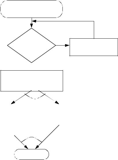
• The next is a flowchart for partial fraction expansions.
start with a function that has a polynomial numerator and denominator
is the order of the
numerator >= yes denominator?
 no
no
Find roots of the denominator and break the equation into partial fraction form with unknown values
use long division to reduce the order of the numerator
|
OR |
|
use limits technique. |
|
use algebra technique |
If there are higher order |
|
|
roots (repeated terms) |
|
|
then derivatives will be |
|
|
|
|
|
required to find solutions |
|
|
|
|
|
Done
• The partial fraction expansion for,

page 13
x(s ) = |
1 |
|
|
|
= |
|
A |
|
+ |
B |
+ |
|
|
|
C |
|
|
|
|
|
|
|
|
|
|
||||||||||||||
|
|
|
|
|
|
|
|
|
|
---- |
--s |
s-----------+ 1 |
|
|
|
|
|
|
|
|
|
|
|||||||||||||||||
|
s2(s + 1 ) s2 |
|
|
|
|
|
|
|
|
|
|
|
|
|
|||||||||||||||||||||||||
C = |
lim |
|
|
|
|
|
|
|
|
|
|
|
|
|
|
1 |
|
|
|
|
= 1 |
|
|
|
|
|
|
|
|
|
|||||||||
|
|
|
|
|
|
|
|
|
|
|
|
|
|
|
|
|
|
|
|
|
|
|
|
|
|||||||||||||||
|
|
(s + 1 ) --------------------- |
|
|
2 |
|
|
|
|
|
|
|
|
|
|
|
|
|
|
|
|
||||||||||||||||||
|
|
|
|
|
|
|
|
|
|
|
|
|
|
|
|
|
|
|
|
|
|
|
|
|
|
|
|
|
|
|
|
|
|
|
|||||
|
s → |
–1 |
|
|
|
|
|
|
|
|
s |
|
|
(s + 1 ) |
|
|
|
|
|
|
|
|
|
|
|
|
|
|
|
||||||||||
|
|
|
|
|
|
|
|
|
|
|
|
|
|
|
|
|
|
|
|
|
|
|
|
|
|
||||||||||||||
A = |
lim |
|
|
s |
2 |
|
|
|
1 |
|
|
|
|
|
|
|
= |
lim |
|
1 |
|
|
= 1 |
|
|
|
|
||||||||||||
|
|
|
|
|
|
|
|
|
|
|
|
|
|
|
|
|
|
||||||||||||||||||||||
|
|
|
|
--------------------- |
2 |
|
|
|
|
|
|
|
|
|
|
----------- |
|
|
|
|
|
|
|||||||||||||||||
|
s → 0 |
|
|
|
|
s |
|
|
(s + 1 ) |
|
|
|
s → 0 |
|
s + 1 |
|
|
|
|
|
|
|
|
|
|||||||||||||||
|
|
|
|
|
|
|
|
|
|
|
|
|
|
|
|
|
|
|
|||||||||||||||||||||
B = lim |
|
|
d |
|
|
s |
2 |
|
|
|
|
|
|
1 |
|
|
|
|
|
|
= |
lim |
|
|
d |
1 |
|
|
= |
–2 |
|||||||||
|
|
|
|
|
|
|
|
|
|
|
|
|
|
|
|
|
|
||||||||||||||||||||||
----- |
|
|
|
--------------------- |
|
2 |
|
|
|
|
|
|
|
|
|
---- |
----------- |
|
lim [–(s + 1 ) ]= –1 |
||||||||||||||||||||
|
|
|
|
|
|
|
|
|
|
|
|
|
|
|
|
|
|
|
|
|
|
|
|
|
|
|
|
|
|
|
|
||||||||
|
s → 0 |
|
ds |
|
|
|
|
s |
|
|
(s + 1 ) |
|
|
|
|
|
s → 0 |
|
|
ds s + 1 |
|
|
|
s → 0 |
|||||||||||||||
|
|
|
|
|
|
|
|
|
|
|
|
|
|
|
|
|
|
||||||||||||||||||||||
• Consider the example below where the order of the numerator is larger than the denominator.
( ) 5s3 + 3s2 + 8s + 6 x s = -------------------------------------------
s2 + 4
This cannot be solved using partial fractions because the numerator is 3rd order and the denominator is only 2nd order. Therefore long division can be used to reduce the order of the equation.
5s + 3
s2 + 4 5s3 + 3s2 + 8s + 6 5s3 + 20s
3s2 – 12s + 6
3s2 + 12
– 12s – 6
This can now be used to write a new function that has a reduced portion that can be solved with partial fractions.
x(s ) = 5s + 3 + |
–---------------------12s – 6 |
solve |
–---------------------12s – 6 |
= |
-------------A |
+ |
------------B |
||||
|
s |
2 |
+ 4 |
|
s |
2 |
+ 4 |
|
s + 2j |
|
s – 2j |
|
|
|
|
|
|
|
|
||||
• When the order of the denominator terms is greater than 1 it requires an expanded partial fraction form, as shown below.