

TsOS / DSP_guide_Smith / Ch30
.pdfChapter 30Complex Numbers |
561 |
added. As you would hope, the third complex number represents the third sinusoid. The complex addition matches the physical system.
Now, imagine multiplying the complex numbers A and B, resulting in another complex number. Does this match what happens when the two sinusoids are multiplied? No! Multiplying two sinusoids does not produce another sinusoid. Complex multiplication fails to match the physical system, and therefore cannot be used.
Fortunately, the valid operations are clearly defined. Two conditions must be satisfied. First, all of the sinusoids must be at the same frequency. For example, if the complex numbers: 1 % 1 j and 2 % 2 j represent sinusoids at the same frequency, then the sum of the two sinusoids is represented by the complex number: 3 % 3 j . However, if 1 % 1 j and 2 % 2 j represent sinusoids with different frequencies, there is nothing that can be done with the complex representation. In this case, the sum of the complex numbers, 3 % 3 j , is meaningless.
In spite of this, frequency can be left as a variable when using complex numbers, but it must be the same frequency everywhere. For instance, it is perfectly valid to add: 2T% 3Tj and 3T% 1 j , to produce: 5T% (3T% 1) j . These represent sinusoids where the amplitude and phase vary as frequency changes. While we do not know what the particular frequency is, we do know that it is the same everywhere, i.e., T.
The second requirement is that the operations being represented must be linear, as discussed in Chapter 5. For instance, sinusoids can be combined by addition and subtraction, but not by multiplication or division. Likewise, systems may be amplifiers, attenuators, high or low-pass filters, etc., but not such actions as: squaring, clipping and thresholding. Remember, even convolution and Fourier analysis are only valid for linear systems.
Complex Representation of Systems
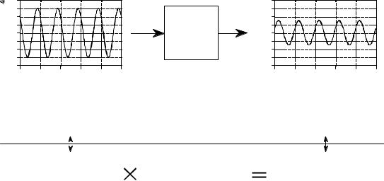
Figure 30-4 shows an example of using complex numbers to represent a sinusoid passing through a linear system. We will use continuous signals for this example, although discrete signals are handled the same way. Since the input signal is a sinusoid, and the system is linear, the output will also be a sinusoid, and at the same frequency as the input. As shown, the example input signal has a conventional representation of: 3 cos(Tt % B/4), o r t h e e q u i v a l e n t e x p r e s s i o n : 2.1213 cos(Tt ) & 2.1213 sin(Tt ) . When represented by a complex number this becomes: 3 e or 2.1213 % j 2.1213 . Likewise, the conventional representation of the output is: 1.5 cos(Tt & B/8), or in the alternate form: 1.3858 cos(Tt ) % 0.5740 sin (Tt ). This is represented by the complex number: 1.5 e or 1.3858 & j 0.5740 .
The system's characteristics can also be represented by a complex number. The magnitude of the complex number is the ratio between the magnitudes
562 |
The Scientist and Engineer's Guide to Digital Signal Processing |
|
|
Input signal |
Output signal |
|
|
4 |
|
|
|
|
|
|
|
3 |
|
|
|
|
|
|
Amplitude |
2 |
|
|
|
|
|
|
1 |
|
|
|
|
|
|
|
|
|
|
|
|
|
|
|
|
0 |
|
|
|
|
|
|
|
-1 |
|
|
|
|
|
|
|
-2 |
|
|
|
|
|
|
|
-3 |
|
|
|
|
|
|
|
-4 |
|
|
|
|
|
|
|
0 |
1 |
2 |
3 |
4 |
5 |
Conventional |
|
|
|
Time |
|
|
|
|
|
3 cos(Tt |
% B/4) |
|
|
||
|
|
|
|
|
|||
|
|
|
|
or |
|
|
|
|
|
2.1213 cos(Tt ) & 2.1213 sin (Tt ) |
|||||
Complex representation |
|
|
|
3 e & jB/4 |
|||
|
|||
|
or |
||
|
2.1213 % j 2.1213 |
||
Linear
System
0.5 e j3B/ 8
or
0.1913 & j 0.4619
|
4 |
|
|
|
|
|
|
3 |
|
|
|
|
|
Amplitude |
2 |
|
|
|
|
|
1 |
|
|
|
|
|
|
|
|
|
|
|
|
|
|
0 |
|
|
|
|
|
|
-1 |
|
|
|
|
|
|
-2 |
|
|
|
|
|
|
-3 |
|
|
|
|
|
|
-4 |
|
|
|
|
|
|
0 |
1 |
2 |
3 |
4 |
5 |
|
|
|
|
Time |
|
|
|
|
1.5 cos(Tt & B/8) |
|
|
||
or
1.3858 cos(Tt ) % 0.5740 sin (Tt )
1.5 e jB/ 8
or
1.3858 & j 0.5740
FIGURE 30-4
Sinusoids represented by complex numbers. Complex numbers are popular in DSP and electronics because they are a convenient way to represent and manipulate sinusoids. As shown in this example, sinusoidal input and output signals can be represented as complex numbers, expressed in either polar or rectangular form. In addition, the change that a linear system makes to a sinusoid can also be expressed as a complex number.
of the input and output (i.e., Mout /Min ). Likewise, the angle of the complex number is the negative of the difference between the input and output angles
(i.e., & [Nout & Nin ]). In the example used here, the system is described by the complex number, 0.5 e j 3B/8 . In other words, the amplitude of the sinusoid is
reduced by 0.5, while the phase angle is changed by & 3B/8 .
The complex number representing the system can be converted into rectangular form as: 0.1913 & j 0.4619 , but we must be careful in interpreting what this means. It does not mean that a sine wave passing through the system is changed in amplitude by 0.1913, nor that a cosine wave is changed by -0.4619. In general, a pure sine or cosine wave entering a linear system is converted into a mixture of sine and cosine waves.
Fortunately, the complex math automatically keeps track of these cross-terms. When a sinusoid passes through a linear system, the complex numbers representing the input signal and the system are multiplied, producing the complex number representing the output. If any two of the complex numbers are known, the third can be found. The calculations can be carried out in either polar or rectangular form, as shown in Fig. 30-4.
In previous chapters we described how the Fourier transform decomposes a signal into cosine and sine waves. The amplitudes of the cosine waves are called the real part, while the amplitudes of the sine waves are called the imaginary part. We stressed that these amplitudes are ordinary numbers, and
Chapter 30Complex Numbers |
563 |
the terms real and imaginary are just names used to keep the two separate. Now that complex numbers have been introduced, it should be quite obvious were the names come from. For example, imagine a 1024 point signal being decomposed into 513 cosine waves and 513 sine waves. Using substitution, we can represent the spectrum by 513 complex numbers. However, don't be misled into thinking that this is the complex Fourier transform, the topic of Chapter 31. This is still the real Fourier transform; the spectrum has just been placed in a complex format by using substitution.
Electrical Circuit Analysis
This method of substituting complex numbers for cosine & sine waves is called the Phasor transform. It is the main tool used to analyze networks composed of resistors, capacitors and inductors. [More formally, electrical engineers define the phasor transform as multiplying by the complex term: e jTt and taking the real part. This allows the procedure to be written as an equation, making it easier to deal with in mathematical work. “Substitution” achieves the same end result, but is less elegant].
The first step is to understand the relationship between the current and voltage for each of these devices. For the resistor, this is expressed in Ohm's law: v ' iR , where i is the instantaneous current through the device, v is the instantaneous voltage across the device, and R is the resistance. In contrast, the capacitor and inductor are governed by the differential equations: i ' C dv /dt , and v ' L di /dt , where C is the capacitance and L is the inductance. In the most general method of circuit analysis, these nasty differential equations are combined as dictated by the circuit configuration, and then solved for the parameters of interest. While this will answer everything about the circuit, the math can become a real mess.
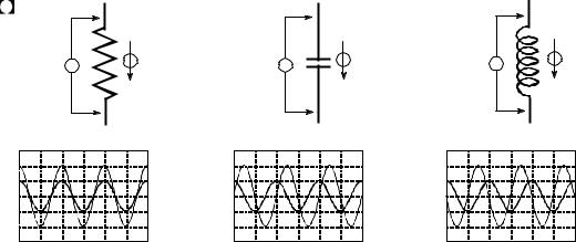
This can be greatly simplified by restricting the signals to be sinusoids. By representing these sinusoids with complex numbers, the difficult differential equations can be directly replaced with much simpler algebraic equations. Figure 30-5 illustrates how this works. We treat each of these three components (resistor, capacitor & inductor) as a system. The input to the system is the sinusoidal current through the device, while the output is the sinusoidal voltage across its two terminals. This means we can represent the input and output of the system by the two complex variables: I (for current) and V (for voltage), respectively. The relation between the input and output can also be expressed by a complex number. This complex number is called the impedance, and is given the symbol: Z. This means:
I × Z ' V
In words, the complex number representing the sinusoidal voltage is equal to the complex number representing the sinusoidal current multiplied by the impedance (another complex number). Given any two, the third can be
564 |
The Scientist and Engineer's Guide to Digital Signal Processing |
|
Resistor |
Capacitor |
Inductor |
V |
I |
V |
I |
V |
I |
|
|
|
Amplitude |
V |
|
I |
||
|
||
|
Time |
Amplitude |
V |
|
I |
||
|
||
|
Time |
Amplitude |
I |
|
|
|
V |
|
Time |
FIGURE 30-5
Definition of impedance. When sinusoidal voltages and currents are represented by complex numbers, the ratio between the two is called the impedance, and is denoted by the complex variable, Z. Resistors, capacitors and inductors have impedances of R, & j/ TC , and jTL , respectively.
found. In polar form, the magnitude of the impedance is the ratio between the amplitudes of V and I. Likewise, the phase of the impedance is the phase difference between V and I.
This relation can be thought of as Ohm's law for sinusoids. Ohms's law ( v ' iR ) describes how the resistance relates the instantaneous current and voltage in a resistor. When the signals are sinusoids represented by complex numbers, the relation becomes: V ' IZ . That is, the impedance relates the current and voltage. Resistance is an ordinary number, since it deals with two ordinary numbers. Impedance is a complex number, since it relates two complex numbers. Impedance contains more information than resistance, because it dictates both the amplitudes and the phase angles.
From the differential equations that govern their operation, it can be shown that the impedance of the resistor, capacitor, and inductor are: R, & j /TC , and jTL , respectively. As an example, imagine that the current in each of these components is a unity amplitude cosine wave, as shown in Fig. 30-5. Using substitution, this is represented by the complex number: 1% 0 j . The voltage
across the resistor will be: |
V ' I Z ' (1% 0 j ) R ' R% 0 j . |
In other words, a |
cosine wave of amplitude R. |
The voltage across the capacitor is found to be: |
|
V ' I Z ' (1% 0 j )(& j /TC ) . |
This reduces to: 0 & j /TC , |
a sine wave of |
amplitude, 1/TC . Likewise, the voltage across the inductor can be calculated: V ' I Z ' (1% 0 j ) ( j TL ) . This reduces to: 0 % j TL , a negative sine wave of amplitude, TL .
The beauty of this method is that RLC circuits can be analyzed without having to resort to differential equations. The impedance of the resistors, capacitors,
Chapter 30Complex Numbers |
565 |
|
Vin |
|||
|
|
|
|
|
|
|
|
|
|
|
|
Z1 |
||
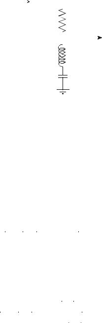
FIGURE 30-6 |
|
|
Vout |
|
|
|
|||
RLC notch filter. This circuit removes a |
|
|
|
|
|
|
|
|
|
narrow band of frequencies from a signal. |
|
|
|
|
|
|
|
|
|
The use of complex substitution greatly |
|
Z2 |
||
simplifies the analysis of this and similar |
|
|||
circuits.
Z3
and inductors is treated the same as resistance in a DC circuit. This includes all of the basic combinations, such as: resistors in series, resistors in parallel, voltage dividers, etc.
As an example, Fig. 30-6 shows an RLC circuit called a notch filter, used to remove a narrow band of frequencies. For instance, it could eliminate 60 hertz interference in an audio or instrumentation signal. If this circuit were composed of three resistors (instead of the resistor, capacitor and inductor), the relationship between the input and output signals would be given by the voltage
divider formula: vout / vin ' (R2% R3 ) /(R1% R2% R3) . Since the circuit contains capacitors and inductors, the equation is rewritten with impedances:
Vout |
' |
Z2 % Z3 |
|
Z1 % Z2 % Z3 |
|
Vin |
||
where: Vout, Vin, Z1, Z2, and Z3 are all complex variables. Plugging in the impedance of each component:
|
|
j TL & |
j |
|
|
|
Vout |
' |
TC |
|
|
||
|
|
|
||||
|
|
|
|
j |
||
Vin |
R % j TL & |
|
||||
|
|
|
|
|
||
TC
Next, we crank through the algebra to separate everything containing a j, from everything that does not contain a j. In other words, we separate the equation into its real and imaginary parts. This algebra can be tiresome and long, but the alternative is to write and solve differential equations, an
566 |
The Scientist and Engineer's Guide to Digital Signal Processing |
Amplitude
1.5
a. Magnitude
1.0 


0.5 


0.0
0.0 |
0.5 |
1.0 |
1.5 |
2.0 |
Frequency (MHz)
|
2 |
|
|
|
|
|
|
b. Phase |
|
|
|
|
1 |
|
|
|
|
(radians) |
0 |
|
|
|
|
Phase |
-1 |
|
|
|
|
|
|
|
|
|
|
|
-2 |
|
|
|
|
|
0.0 |
0.5 |
1.0 |
1.5 |
2.0 |
Frequency (MHz)
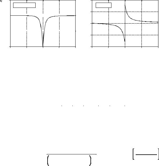
FIGURE 30-7
Notch filter frequency response. These curves are for the component values: R = 50S, C = 470DF, and L = 54 µH.
even nastier task. When separated into the real and imaginary parts, the complex representation of the notch filter becomes:
Vout |
' |
k 2 |
% |
j |
R k |
|
Vin |
R 2% k 2 |
R 2% k 2 |
||||
|
|
|
where: k ' TL & 1/TC
Lastly, the relation is converted to polar notation, and graphed in Fig. 30-7:
Mag ' |
TL & 1/TC |
Phase ' |
arctan |
R |
|
TL & 1/TC |
|||
|
R 2 % [ TL & 1/TC ] 2 |
1/2 |
|
|
|
|
|
||
|
|
|
|
The key point to remember from these examples is how substitution allows complex numbers to represent real world problems. In the next chapter we will look at a more advanced way to use complex numbers in science and engineering, mathematical equivalence.