

486 |
The Scientist and Engineer's Guide to Digital Signal Processing |
Example Encoding Table
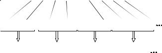
FIGURE 27-3
Huffman encoding. The encoding table assigns each of the seven letters used in this example a variable length binary code, based on its probability of occurrence. The original data stream composed of these 7 characters is translated by this table into the Huffman encoded data. Since each of the Huffman codes is a different length, the binary data need to be regrouped into standard 8 bit bytes for storage and transmission.
original data stream:
letter |
|
probability |
|
Huffman code |
|
|
|||
A |
|
.154 |
|
1 |
B |
|
.110 |
|
01 |
C |
|
.072 |
|
0010 |
D |
|
.063 |
|
0011 |
E |
|
.059 |
|
0001 |
F |
|
.015 |
|
000010 |
G |
|
.011 |
|
000011 |
|
|
|
|
|
C E G A D F B E A 


Huffman encoded: |
0010 0001 |
000011 1 0011 000010 01 00 01 1 |
||
grouped into bytes: |
00100001 |
00001110 01100001 00100011 |
||
|
byte 1 |
byte 2 |
byte 3 |
byte 4 |
looks at the stream of ones and zeros until a valid code is formed, and then starting over looking for the next character. The way that the codes are formed insures that no ambiguity exists in the separation.
A more sophisticated version of the Huffman approach is called arithmetic encoding. In this scheme, sequences of characters are represented by individual codes, according to their probability of occurrence. This has the advantage of better data compression, say 5-10%. Run-length encoding followed by either Huffman or arithmetic encoding is also a common strategy. As you might expect, these types of algorithms are very complicated, and usually left to data compression specialists.
To implement Huffman or arithmetic encoding, the compression and uncompression algorithms must agree on the binary codes used to represent each character (or groups of characters). This can be handled in one of two ways. The simplest is to use a predefined encoding table that is always the same, regardless of the information being compressed. More complex schemes use encoding optimized for the particular data being used. This requires that the encoding table be included in the compressed file for use by the uncompression program. Both methods are common.
Delta Encoding
In science, engineering, and mathematics, the Greek letter delta ()) is used to denote the change in a variable. The term delta encoding, refers to
|
|
|
|
Chapter 27Data Compression |
487 |
|
original data stream: |
17 19 24 24 24 21 15 10 89 |
95 96 96 96 95 94 94 95 93 90 87 86 86 |
||||
|
move |
delta |
delta |
delta |
|
|
delta encoded: |
17 |
2 |
5 |
0 0 -3 -6 -5 79 |
6 1 0 0 -1 -1 0 |
1 -2 -3 -3 -1 0 |
FIGURE 27-4
Example of delta encoding. The first value in the encoded file is the same as the first value in the original file. Thereafter, each sample in the encoded file is the difference between the current and last sample in the original file.
several techniques that store data as the difference between successive samples (or characters), rather than directly storing the samples themselves. Figure 27- 4 shows an example of how this is done. The first value in the delta encoded file is the same as the first value in the original data. All the following values in the encoded file are equal to the difference (delta) between the corresponding value in the input file, and the previous value in the input file.
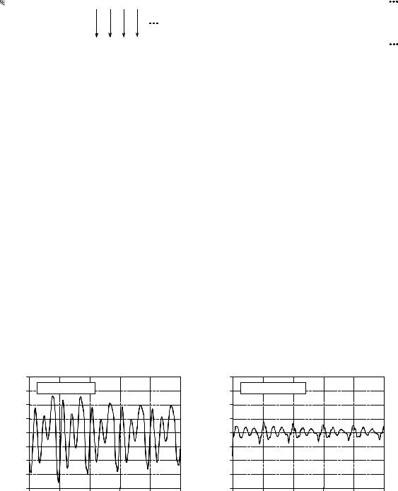
Delta encoding can be used for data compression when the values in the original data are smooth, that is, there is typically only a small change between adjacent values. This is not the case for ASCII text and executable code; however, it is very common when the file represents a signal. For instance, Fig. 27-5a shows a segment of an audio signal, digitized to 8 bits, with each sample between -127 and 127. Figure 27-5b shows the delta encoded version of this signal. The key feature is that the delta encoded signal has a lower amplitude than the original signal. In other words, delta encoding has increased the probability that each sample's value will be near zero, and decreased the probability that it will be far from zero. This uneven probability is just the thing that Huffman encoding needs to operate. If the original signal is not changing, or is changing in a straight line, delta encoding will result in runs of samples having the same value.
|
128 |
|
|
|
|
|
|
96 |
a. Audio signal |
|
|
|
|
|
|
|
|
|
|
|
|
64 |
|
|
|
|
|
mplitudeA |
32 |
|
|
|
|
|
-32 |
|
|
|
|
|
|
|
0 |
|
|
|
|
|
|
-64 |
|
|
|
|
|
|
-96 |
|
|
|
|
|
|
-128 |
|
|
|
|
|
|
0 |
100 |
200 |
300 |
400 |
500 |
Sample number
|
128 |
|
|
|
|
|
|
96 |
b. Delta encoded |
|
|
|
|
|
|
|
|
|
|
|
|
64 |
|
|
|
|
|
Amplitude |
32 |
|
|
|
|
|
-32 |
|
|
|
|
|
|
|
0 |
|
|
|
|
|
|
-64 |
|
|
|
|
|
|
-96 |
|
|
|
|
|
|
-128 |
|
|
|
|
|
|
0 |
100 |
200 |
300 |
400 |
500 |
Sample number
FIGURE 27-5
Example of delta encoding. Figure (a) is an audio signal digitized to 8 bits. Figure (b) shows the delta encoded version of this signal. Delta encoding is useful for data compression if the signal being encoded varies slowly from sample-to-sample.
488 |
The Scientist and Engineer's Guide to Digital Signal Processing |
This is what run-length encoding requires. Correspondingly, delta encoding followed by Huffman and/or run-length encoding is a common strategy for compressing signals.
The idea used in delta encoding can be expanded into a more complicated technique called Linear Predictive Coding, or LPC. To understand LPC, imagine that the first 99 samples from the input signal have been encoded, and we are about to work on sample number 100. We then ask ourselves: based on the first 99 samples, what is the most likely value for sample 100? In delta encoding, the answer is that the most likely value for sample 100 is the same as the previous value, sample 99. This expected value is used as a reference to encode sample 100. That is, the difference between the sample and the expectation is placed in the encoded file. LPC expands on this by making a better guess at what the most probable value is. This is done by looking at the last several samples, rather than just the last sample. The algorithms used by LPC are similar to recursive filters, making use of the z-transform and other intensively mathematical techniques.
LZW Compression
LZW compression is named after its developers, A. Lempel and J. Ziv, with later modifications by Terry A. Welch. It is the foremost technique for general purpose data compression due to its simplicity and versatility. Typically, you can expect LZW to compress text, executable code, and similar data files to about one-half their original size. LZW also performs well when presented with extremely redundant data files, such as tabulated numbers, computer source code, and acquired signals. Compression ratios of 5:1 are common for these cases. LZW is the basis of several personal computer utilities that claim to "double the capacity of your hard drive."
LZW compression is always used in GIF image files, and offered as an option in TIFF and PostScript. LZW compression is protected under U.S. patent number 4,558,302, granted December 10, 1985 to Sperry Corporation (now the Unisys Corporation). For information on commercial licensing, contact: Welch Licensing Department, Law Department, M/SC2SW1, Unisys Corporation, Blue Bell, Pennsylvania, 19424-0001.
LZW compression uses a code table, as illustrated in Fig. 27-6. A common choice is to provide 4096 entries in the table. In this case, the LZW encoded data consists entirely of 12 bit codes, each referring to one of the entries in the code table. Uncompression is achieved by taking each code from the compressed file, and translating it through the code table to find what character or characters it represents. Codes 0-255 in the code table are always assigned to represent single bytes from the input file. For example, if only these first 256 codes were used, each byte in the original file would be converted into 12 bits in the LZW encoded file, resulting in a 50% larger file size. During uncompression, each 12 bit code would be translated via the code table back into the single bytes. Of course, this wouldn't be a useful situation.
Chapter 27Data Compression |
489 |
Example Code Table
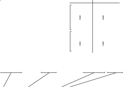
FIGURE 27-6
Example of code table compression. This is the basis of the popular LZW compression method. Encoding occurs by identifying sequences of bytes in the original file that exist in the code table. The 12 bit code representing the sequence is placed in the compressed file instead of the sequence. The first 256 entries in the table correspond to the single byte values, 0 to 255, while the remaining entries correspond to sequences of bytes. The LZW algorithm is an efficient way of generating the code table based on the particular data being compressed. (The code table in this figure is a simplified example, not one actually generated by the LZW algorithm).
unique code identical code
code number
0000
0001
0254
0255
0256
0257
4095
translation
0
1
254
255
145 201 4
243245
xxxxxx xxx
original data stream: 123 145 201 4 119 89 243 245 59 11 206 145 201 4 243 245 


code table encoded: 123 256 119 89 257 59 11 206 256 257


The LZW method achieves compression by using codes 256 through 4095 to represent sequences of bytes. For example, code 523 may represent the sequence of three bytes: 231 124 234. Each time the compression algorithm encounters this sequence in the input file, code 523 is placed in the encoded file. During uncompression, code 523 is translated via the code table to recreate the true 3 byte sequence. The longer the sequence assigned to a single code, and the more often the sequence is repeated, the higher the compression achieved.
Although this is a simple approach, there are two major obstacles that need to be overcome: (1) how to determine what sequences should be in the code table, and (2) how to provide the uncompression program the same code table used by the compression program. The LZW algorithm exquisitely solves both these problems.
When the LZW program starts to encode a file, the code table contains only the first 256 entries, with the remainder of the table being blank. This means that the first codes going into the compressed file are simply the single bytes from the input file being converted to 12 bits. As the encoding continues, the LZW algorithm identifies repeated sequences in the data, and adds them to the code table. Compression starts the second time a sequence is encountered. The key point is that a sequence from the input file is not added to the code table until it has already been placed in the compressed file as individual characters (codes 0 to 255). This is important because it allows the uncompression program to reconstruct the code table directly from the compressed data, without having to transmit the code table separately.
490 |
The Scientist and Engineer's Guide to Digital Signal Processing |
|||||
|
|
|
START |
|
|
|
|
|
|
|
1 |
|
|
|
|
|
|
|
|
|
|
|
|
input first byte, |
|
||
|
|
|
store in STRING |
|
|
|
|
|
|
|
2 |
|
|
|
|
|
|
|
|
|
|
|
|
input next byte, |
|
||
|
|
|
store in CHAR |
|
|
|
|
|
|
|
3 |
|
|
|
|
|
|
|
|
|
|
|
NO |
is |
|
||
|
|
STRING+CHAR |
YES |
|
||
|
|
|
|
|
||
|
|
|
in table? |
|
|
|
|
output the code |
4 |
|
STRING = |
7 |
|
|
for STRING |
|
|
STRING + CHAR |
|
|
|
|
5 |
|
|
|
|
|
|
|
|
|
|
|
|
add entry in table for |
|
|
|
||
|
STRING+CHAR |
|
|
|
|
|
6
STRING = CHAR
YES |
more bytes |
8 |
|
|
|||
|
to input? |
|
|
|
|
NO |
9 |
|
|
||
|
|
|
|
|
ouput the code |
||
|
for STRING |
|
|
END
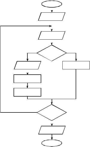
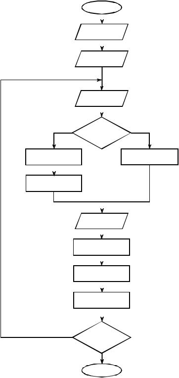
FIGURE 27-7
LZW compression flowchart. The variable, CHAR, is a single byte. The variable, STRING, is a variable length sequence of bytes. Data are read from the input file (box 1 & 2) as single bytes, and written to the compressed file (box 4) as 12 bit codes. Table 27-3 shows an example of this algorithm.
Figure 27-7 shows a flowchart for LZW compression. Table 27-3 provides the step-by-step details for an example input file consisting of 45 bytes, the ASCII text string: the/rain/in/Spain/falls/mainly/on/the/plain. When we say that the LZW algorithm reads the character "a" from the input file, we mean it reads the value: 01100001 (97 expressed in 8 bits), where 97 is "a" in ASCII. When we say it writes the character "a" to the encoded file, we mean it writes: 000001100001 (97 expressed in 12 bits).
|
|
|
|
Chapter 27Data Compression |
491 |
||||
|
|
|
|
|
|
|
|
|
|
|
CHAR |
STRING |
In Table? Output |
Add to |
New |
Comments |
|||
|
+ CHAR |
Table |
STRING |
||||||
|
|
|
|
|
|
||||
1 |
t |
t |
|
|
|
|
|
t |
first characterno action |
2 |
h |
th |
no |
|
t |
256 |
= th |
h |
|
3 |
e |
he |
no |
|
h |
257 |
= he |
e |
|
4 |
/ |
e/ |
no |
|
e |
258 |
= e/ |
/ |
|
5 |
r |
/r |
no |
|
/ |
259 |
= /r |
r |
|
6 |
a |
ra |
no |
|
r |
260 |
= ra |
a |
|
7 |
i |
ai |
no |
|
a |
261 |
= ai |
i |
|
8 |
n |
in |
no |
|
i |
262 |
= in |
n |
|
9 |
/ |
n/ |
no |
|
n |
263 |
= n/ |
/ |
|
10 |
i |
/i |
no |
|
/ |
264 |
= /i |
i |
|
11 |
n |
in |
yes |
(262) |
|
|
|
in |
first match found |
12 |
/ |
in/ |
no |
|
262 |
265 |
= in/ |
/ |
|
13 |
S |
/S |
no |
|
/ |
266 |
= /S |
S |
|
14 |
p |
Sp |
no |
|
S |
267 |
= Sp |
p |
|
15 |
a |
pa |
no |
|
p |
268 |
= pa |
a |
|
16 |
i |
ai |
yes |
(261) |
|
|
|
ai |
matches ai, ain not in table yet |
17 |
n |
ain |
no |
|
261 |
269 |
= ain |
n |
ain added to table |
18 |
/ |
n/ |
yes |
(263) |
|
|
|
n/ |
|
19 |
f |
n/f |
no |
|
263 |
270 |
= n/f |
f |
|
20 |
a |
fa |
no |
|
f |
271 |
= fa |
a |
|
21 |
l |
al |
no |
|
a |
272 |
= al |
l |
|
22 |
l |
ll |
no |
|
l |
273 |
= ll |
l |
|
23 |
s |
ls |
no |
|
l |
274 |
= ls |
s |
|
24 |
/ |
s/ |
no |
|
s |
275 |
= s/ |
/ |
|
25 |
m |
/m |
no |
|
/ |
276 |
= /m |
m |
|
26 |
a |
ma |
no |
|
m |
277 |
= ma |
a |
|
27 |
i |
ai |
yes |
(261) |
|
|
|
ai |
matches ai |
28 |
n |
ain |
yes |
(269) |
|
|
|
ain |
matches longer string, ain |
29 |
l |
ainl |
no |
|
269 |
278 |
= ainl |
l |
|
30 |
y |
ly |
no |
|
l |
279 = ly |
y |
|
|
31 |
/ |
y/ |
no |
|
y |
280 = y/ |
/ |
|
|
32 |
o |
/o |
no |
|
/ |
281 |
= /o |
o |
|
33 |
n |
on |
no |
|
o |
282 = on |
n |
|
|
34 |
/ |
n/ |
yes |
(263) |
|
|
|
n/ |
|
35 |
t |
n/t |
no |
|
263 |
283 |
= n/t |
t |
|
36 |
h |
th |
yes |
(256) |
|
|
|
th |
matches th, the not in table yet |
37 |
e |
the |
no |
|
256 |
284 |
= the |
e |
the added to table |
38 |
/ |
e/ |
yes |
|
|
|
|
e/ |
|
39 |
p |
e/p |
no |
|
258 |
285 |
= e/p |
p |
|
40 |
l |
pl |
no |
|
p |
286 |
= pl |
l |
|
41 |
a |
la |
no |
|
l |
287 |
= la |
a |
|
42 |
i |
ai |
yes |
(261) |
|
|
|
ai |
matches ai |
43 |
n |
ain |
yes |
(269) |
|
|
|
ain |
matches longer string ain |
44 |
/ |
ain/ |
no |
|
269 |
288 |
= ain/ |
/ |
|
45 |
EOF |
/ |
|
|
/ |
|
|
|
end of file, output STRING |
TABLE 27-3
LZW example. This shows the compression of the phrase: the/rain/in/Spain/falls/mainly/on/the/plain/.
492 |
The Scientist and Engineer's Guide to Digital Signal Processing |
The compression algorithm uses two variables: CHAR and STRING. The variable, CHAR, holds a single character, i.e., a single byte value between 0 and 255. The variable, STRING, is a variable length string, i.e., a group of one or more characters, with each character being a single byte. In box 1 of Fig. 27-7, the program starts by taking the first byte from the input file, and placing it in the variable, STRING. Table 27-3 shows this action in line 1. This is followed by the algorithm looping for each additional byte in the input file, controlled in the flow diagram by box 8. Each time a byte is read from the input file (box 2), it is stored in the variable, CHAR. The data table is then searched to determine if the concatenation of the two variables, STRING+CHAR, has already been assigned a code (box 3).
If a match in the code table is not found, three actions are taken, as shown in boxes 4, 5 & 6. In box 4, the 12 bit code corresponding to the contents of the variable, STRING, is written to the compressed file. In box 5, a new code is created in the table for the concatenation of STRING+CHAR. In box 6, the variable, STRING, takes the value of the variable, CHAR. An example of these actions is shown in lines 2 through 10 in Table 27-3, for the first 10 bytes of the example file.
When a match in the code table is found (box 3), the concatenation of STRING+CHAR is stored in the variable, STRING, without any other action taking place (box 7). That is, if a matching sequence is found in the table, no action should be taken before determining if there is a longer matching sequence also in the table. An example of this is shown in line 11, where the sequence: STRING+CHAR = in, is identified as already having a code in the table. In line 12, the next character from the input file, /, is added to the sequence, and the code table is searched for: in/. Since this longer sequence is not in the table, the program adds it to the table, outputs the code for the shorter sequence that is in the table (code 262), and starts over searching for sequences beginning with the character, /. This flow of events is continued until there are no more characters in the input file. The program is wrapped up with the code corresponding to the current value of STRING being written to the compressed file (as illustrated in box 9 of Fig. 27-7 and line 45 of Table 27-3).
A flowchart of the LZW uncompression algorithm is shown in Fig. 27-8. Each code is read from the compressed file and compared to the code table to provide the translation. As each code is processed in this manner, the code table is updated so that it continually matches the one used during the compression. However, there is a small complication in the uncompression routine. There are certain combinations of data that result in the uncompression algorithm receiving a code that does not yet exist in its code table. This contingency is handled in boxes 4,5 & 6.
Only a few dozen lines of code are required for the most elementary LZW programs. The real difficulty lies in the efficient management of the code table. The brute force approach results in large memory requirements and a slow program execution. Several tricks are used in commercial LZW programs to improve their performance. For instance, the memory problem
Chapter 27Data Compression |
493 |
||
START |
|
|
|
|
1 |
|
|
|
|
|
|
input first code, |
|
||
store in OCODE |
|
|
|
|
2 |
|
|
|
|
|
|
output translation |
|
||
of OCODE |
|
|
|
|
|
input next code, |
3 |
|
|
|
|
store in NCODE |
|
|
|
|
|
|
|
4 |
|
|
|
|
|
|
|
|
NO |
is |
|
||
|
YES |
|
|||
|
|
NCODE in table? |
|
|
|
STRING = |
5 |
|
STRING = |
7 |
|
translation of OCODE |
|
|
translation of NCODE |
|
|
|
6 |
|
|
|
|
|
|
|
|
|
|
STRING = |
|
|
|
||
STRING+CHAR |
|
|
|
|
|
|
|
|
|
8 |
|
|
|
|
|
|
|
|
|
ouput STRING |
|
||
|
|
|
|
||
|
|
|
9 |
|
|
|
|
|
|
|
|
|
|
CHAR = the first |
|
||
|
character in STRING |
|
|||
|
|
|
|
||
|
|
|
|
|
|
|
|
add entry in table for 10 |
|
||
|
|
OCODE + CHAR |
|
|
|
|
|
|
|
11 |
|
|
|
|
|
|
|
|
|
OCODE = NCODE |
|
||
|
|
|
|
||
|
YES |
|
|
12 |
|
|
|
|
|
||
|
more codes |
|
|||
|
|
|
|||
to input?
NO
END
FIGURE 27-8
LZW uncompression flowchart. The variables, OCODE and NCODE (oldcode and newcode), hold the 12 bit codes from the compressed file, CHAR holds a single byte, STRING holds a string of bytes.