

390 |
The Scientist and Engineer's Guide to Digital Signal Processing |
Figure (d) shows the display optimized to view pixel values around digital number 75. This is done by turning up the contrast, resulting in the output transform increasing in slope. For example, the stored pixel values of 71 and 75 become 100 and 116 in the display, making the contrast a factor of four greater. Pixel values between 46 and 109 are displayed as the blackest black, to the whitest white. The price for this increased contrast is that pixel values 0 to 45 are saturated at black, and pixel values 110 to 255 are saturated at white. As shown in (d), the increased contrast allows the triangles in the left square to be seen, at the cost of saturating the middle and right squares.
Figure (e) shows the effect of increasing the contrast even further, resulting in only 16 of the possible 256 stored levels being displayed as nonsaturated. The brightness has also been decreased so that the 16 usable levels are centered on digital number 175. The details in the center square are now very visible; however, almost everything else in the image is saturated. For example, look at the noise around the border of the image. There are very few pixels with an intermediate gray shade; almost every pixel is either pure black or pure white. This technique of using high contrast to view only a few levels is sometimes called a grayscale stretch.
The contrast adjustment is a way of zooming in on a smaller range of pixel values. The brightness control centers the zoomed section on the pixel values of interest. Most digital imaging systems allow the brightness and contrast to be adjusted in just this manner, and often provide a graphical display of the output transform (as in Fig. 23-12). In comparison, the brightness and contrast controls on television and video monitors are analog circuits, and may operate differently. For example, the contrast control of a monitor may adjust the gain of the analog signal, while the brightness might add or subtract a DC offset. The moral is, don't be surprised if these analog controls don't respond in the way you think they should.
Grayscale Transforms
The last image, Fig. 23-12f, is different from the rest. Rather than having a slope in the curve over one range of input values, it has a slope in the curve over two ranges. This allows the display to simultaneously show the triangles in both the left and the right squares. Of course, this results in saturation of the pixel values that are not near these digital numbers. Notice that the slide bars for contrast and brightness are not shown in (f); this display is beyond what brightness and contrast adjustments can provide.
Taking this approach further results in a powerful technique for improving the appearance of images: the grayscale transform. The idea is to increase the contrast at pixel values of interest, at the expense of the pixel values we don't care about. This is done by defining the relative importance of each of the 0 to 255 possible pixel values. The more important the value, the greater its contrast is made in the displayed image. An example will show a systematic way of implementing this procedure.

a. Normal
B
C
b. Increased brightness
B
C
c. Decreased brightness
B
C
d.Slightly increased contrast at DN 75
B
C
e.Greatly increased contrast at DN 150
B
C
f.Increased contrast at both DN 75 and 225
B
C
|
Chapter 23Image Formation and Display |
391 |
|||||
value |
250 |
|
|
|
|
|
|
200 |
|
|
|
|
|
|
|
Output |
150 |
|
|
|
|
|
|
100 |
|
|
|
|
|
|
|
|
|
|
|
|
|
|
|
|
50 |
|
|
|
|
|
|
|
0 |
|
|
|
|
|
|
|
0 |
50 |
100 |
150 |
200 |
250 |
|
|
|
|
Input value |
|
|
|
|
value |
250 |
|
|
|
|
|
200 |
|
|
|
|
|
|
|
|
|
|
|
|
|
Output |
150 |
|
|
|
|
|
100 |
|
|
|
|
|
|
|
50 |
|
|
|
|
|
|
0 |
|
|
|
|
|
|
0 |
50 |
100 |
150 |
200 |
250 |
|
|
|
Input value |
|
|
|
value |
250 |
|
|
|
|
|
200 |
|
|
|
|
|
|
|
|
|
|
|
|
|
Output |
150 |
|
|
|
|
|
100 |
|
|
|
|
|
|
|
|
|
|
|
|
|
|
50 |
|
|
|
|
|
|
0 |
|
|
|
|
|
|
0 |
50 |
100 |
150 |
200 |
250 |
|
|
|
Input value |
|
|
|
value |
250 |
|
|
|
|
|
200 |
|
|
|
|
|
|
|
|
|
|
|
|
|
Output |
150 |
|
|
|
|
|
100 |
|
|
|
|
|
|
|
|
|
|
|
|
|
|
50 |
|
|
|
|
|
|
0 |
|
|
|
|
|
|
0 |
50 |
100 |
150 |
200 |
250 |
|
|
|
Input value |
|
|
|
value |
250 |
|
|
|
|
|
200 |
|
|
|
|
|
|
|
|
|
|
|
|
|
Output |
150 |
|
|
|
|
|
100 |
|
|
|
|
|
|
|
|
|
|
|
|
|
|
50 |
|
|
|
|
|
|
0 |
|
|
|
|
|
|
0 |
50 |
100 |
150 |
200 |
250 |
|
|
|
Input value |
|
|
|
value |
250 |
|
|
|
|
|
200 |
|
|
|
|
|
|
Output |
150 |
|
|
|
|
|
100 |
|
|
|
|
|
|
|
|
|
|
|
|
|
|
50 |
|
|
|
|
|
|
0 |
|
|
|
|
|
|
0 |
50 |
100 |
150 |
200 |
250 |
Input value
FIGURE 23-12
392 |
The Scientist and Engineer's Guide to Digital Signal Processing |
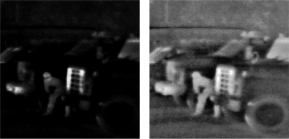
a. Original IR image |
b. With grayscale transform |
FIGURE 23-13
Grayscale processing. Image (a) was acquired with an infrared camera in total darkness. Brightness in the image is related to the temperature, accounting for the appearance of the warm human body and the hot truck grill. Image (b) was processed with the manual grayscale transform shown in Fig. 23-14c.
The image in Fig. 23-13a was acquired in total darkness by using a CCD camera that is sensitive in the far infrared. The parameter being imaged is temperature: the hotter the object, the more infrared energy it emits and the brighter it appears in the image. This accounts for the background being very black (cold), the body being gray (warm), and the truck grill being white (hot). These systems are great for the military and police; you can see the other guy when he can't even see himself! The image in (a) is difficult to view because of the uneven distribution of pixel values. Most of the image is so dark that details cannot be seen in the scene. On the other end, the grill is near white saturation.
The histogram of this image is displayed in Fig. 23-14a, showing that the background, human, and grill have reasonably separate values. In this example, we will increase the contrast in the background and the grill, at the expense of everything else, including the human body. Figure (b) represents this strategy. We declare that the lowest pixel values, the background, will have a relative contrast of twelve. Likewise, the highest pixel values, the grill, will have a relative contrast of six. The body will have a relative contrast of one, with a staircase transition between the regions. All these values are determined by trial and error.
The grayscale transform resulting from this strategy is shown in (c), labeled manual. It is found by taking the running sum (i.e., the discrete integral) of the curve in (b), and then normalizing so that it has a value of 255 at the
Chapter 23Image Formation and Display |
393 |
|
1600 |
|
|
|
|
|
|
1400 |
a. Histogram |
|
|
|
|
pixelsof |
1200 |
background |
|
|
|
|
1000 |
|
|
|
|
|
|
|
|
|
|
|
|
|
Number |
800 |
|
|
|
|
|
600 |
|
|
|
|
|
|
|
|
|
|
|
|
|
|
400 |
|
human body |
|
|
|
|
|
|
|
|
|
|
|
200 |
|
|
|
|
grill |
|
0 |
|
|
|
|
|
|
0 |
50 |
100 |
150 |
200 |
250 |
Value of pixel
FIGURE 23-14
Developing a grayscale transform. Figure (a) is the histogram of the raw image in Fig. 23-13a. In (b), a curve is manually generated indicating the desired contrast at each pixel value. The LUT for the output transform is then found by integration and normalization of (b), resulting in the curve labeled manual in (c). In histogram equalization, the histogram of the raw image, shown in (a), is integrated and normalized to find the LUT, shown in (c).
16
14 
 b. Desired contrast
12
contrast |
10 |
|
|
||
Desired |
8 |
|
6 |
||
|
||
|
4 |
|
|
2 |
|
|
0 |
0 |
50 |
100 |
150 |
200 |
250 |
Value of pixel
|
250 |
|
|
|
|
|
|
|
|
from histogram |
|
|
|
|
200 |
|
|
|
|
|
value |
|
|
|
manual |
|
|
150 |
|
|
|
|
|
|
Display |
|
|
|
|
|
|
100 |
|
|
|
|
|
|
|
|
|
|
|
|
|
|
50 |
|
|
c. Output transform |
|
|
|
0 |
|
|
|
|
|
|
0 |
50 |
100 |
150 |
200 |
250 |
Input value
right side. Why take the integral to find the required curve? Think of it this way: The contrast at a particular pixel value is equal to the slope of the output transform. That is, we want (b) to be the derivative (slope) of (c). This means that (c) must be the integral of (b).
Passing the image in Fig. 23-13a through this manually determined grayscale transform produces the image in (b). The background has been made lighter, the grill has been made darker, and both have better contrast. These improvements are at the expense of the body's contrast, producing a less detailed image of the intruder (although it can't get much worse than in the original image).
Grayscale transforms can significantly improve the viewability of an image. The problem is, they can require a great deal of trial and error. Histogram equalization is a way to automate the procedure. Notice that the histogram in (a) and the contrast weighting curve in (b) have the same general shape. Histogram equalization blindly uses the histogram as the contrast weighing curve, eliminating the need for human judgement. That is, the output transform is found by integration and normalization of the histogram, rather than a manually generated curve. This results in the greatest contrast being given to those values that have the greatest number of pixels.