

TsOS / DSP_guide_Smith / Ch13
.pdfCHAPTER
Continuous Signal Processing
13
Continuous signal processing is a parallel field to DSP, and most of the techniques are nearly identical. For example, both DSP and continuous signal processing are based on linearity, decomposition, convolution and Fourier analysis. Since continuous signals cannot be directly represented in digital computers, don't expect to find computer programs in this chapter. Continuous signal processing is based on mathematics; signals are represented as equations, and systems change one equation into another. Just as the digital computer is the primary tool used in DSP, calculus is the primary tool used in continuous signal processing. These techniques have been used for centuries, long before computers were developed.
The Delta Function
Continuous signals can be decomposed into scaled and shifted delta functions, just as done with discrete signals. The difference is that the continuous delta function is much more complicated and mathematically abstract than its discrete counterpart. Instead of defining the continuous delta function by what it is, we will define it by the characteristics it has.
A thought experiment will show how this works. Imagine an electronic circuit composed of linear components, such as resistors, capacitors and inductors. Connected to the input is a signal generator that produces various shapes of short pulses. The output of the circuit is connected to an oscilloscope, displaying the waveform produced by the circuit in response to each input pulse. The question we want to answer is: how is the shape of the output pulse related to the characteristics of the input pulse? To simplify the investigation, we will only use input pulses that are much shorter than the output. For instance, if the system responds in milliseconds, we might use input pulses only a few microseconds in length.
After taking many measurement, we come to three conclusions: First, the shape of the input pulse does not affect the shape of the output signal. This
243
244 |
The Scientist and Engineer's Guide to Digital Signal Processing |
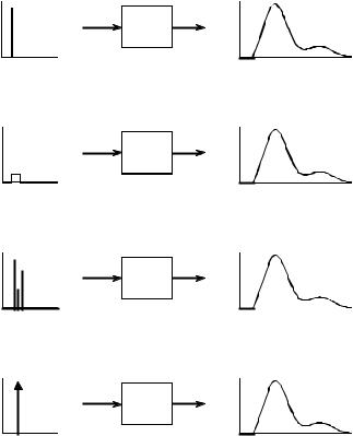
is illustrated in Fig. 13-1, where various shapes of short input pulses produce exactly the same shape of output pulse. Second, the shape of the output waveform is totally determined by the characteristics of the system, i.e., the value and configuration of the resistors, capacitors and inductors. Third, the amplitude of the output pulse is directly proportional to the area of the input pulse. For example, the output will have the same amplitude for inputs of: 1 volt for 1 microsecond, 10 volts for 0.1 microseconds, 1,000 volts for 1 nanosecond, etc. This relationship also allows for input pulses with negative areas. For instance, imagine the combination of a 2 volt pulse lasting 2 microseconds being quickly followed by a -1 volt pulse lasting 4 microseconds. The total area of the input signal is zero, resulting in the output doing nothing.
Input signals that are brief enough to have these three properties are called impulses. In other words, an impulse is any signal that is entirely zero except for a short blip of arbitrary shape. For example, an impulse to a microwave transmitter may have to be in the picosecond range because the electronics responds in nanoseconds. In comparison, a volcano that erupts for years may be a perfectly good impulse to geological changes that take millennia.
Mathematicians don't like to be limited by any particular system, and commonly use the term impulse to mean a signal that is short enough to be an impulse to any possible system. That is, a signal that is infinitesimally narrow. The continuous delta function is a normalized version of this type of impulse. Specifically, the continuous delta function is mathematically defined by three idealized characteristics: (1) the signal must be infinitesimally brief, (2) the pulse must occur at time zero, and (3) the pulse must have an area of one.
Since the delta function is defined to be infinitesimally narrow and have a fixed area, the amplitude is implied to be infinite. Don't let this bother you; it is completely unimportant. Since the amplitude is part of the shape of the impulse, you will never encounter a problem where the amplitude makes any difference, infinite or not. The delta function is a mathematical construct, not a real world signal. Signals in the real world that act as delta functions will always have a finite duration and amplitude.
Just as in the discrete case, the continuous delta function is given the mathematical symbol: *( ) . Likewise, the output of a continuous system in response to a delta function is called the impulse response, and is often denoted by: h ( ) . Notice that parentheses, ( ), are used to denote continuous signals, as compared to brackets, [ ], for discrete signals. This notation is used in this book and elsewhere in DSP, but isn't universal. Impulses are displayed in graphs as vertical arrows (see Fig. 13-1d), with the length of the arrow indicating the area of the impulse.
To better understand real world impulses, look into the night sky at a planet and a star, for instance, Mars and Sirius. Both appear about the same brightness and size to the unaided eye. The reason for this similarity is not
a.
b.
c
Chapter 13Continuous Signal Processing |
245 |
Linear
System
Linear
System
Linear
System
|
*(t) |
|
d. |
Linear |
|
System |
||
|
FIGURE 13-1
The continuous delta function. If the input to a linear system is brief compared to the resulting output, the shape of the output depends only on the characteristics of the system, and not the shape of the input. Such short input signals are called impulses. Figures a,b & c illustrate example input signals that are impulses for this particular system. The term delta function is used to describe a normalized impulse, i.e., one that occurs at t ' 0 and has an area of one. The mathematical symbols for the delta function are shown in (d), a vertical arrow and *(t).
obvious, since the viewing geometry is drastically different. Mars is about 6000 kilometers in diameter and 60 million kilometers from earth. In comparison, Sirius is about 300 times larger and over one-million times farther away. These dimensions should make Mars appear more than three-thousand times larger than Sirius. How is it possible that they look alike?
These objects look the same because they are small enough to be impulses to the human visual system. The perceived shape is the impulse response of the eye, not the actual image of the star or planet. This becomes obvious when the two objects are viewed through a small telescope; Mars appears as a dim disk, while Sirius still appears as a bright impulse. This is also the reason that stars twinkle while planets do not. The image of a star is small enough that it can be briefly blocked by particles or turbulence in the atmosphere, whereas the larger image of the planet is much less affected.
246 |
The Scientist and Engineer's Guide to Digital Signal Processing |
Convolution
Just as with discrete signals, the convolution of continuous signals can be viewed from the input signal, or the output signal. The input side viewpoint is the best conceptual description of how convolution operates. In comparison, the output side viewpoint describes the mathematics that must be used. These descriptions are virtually identical to those presented in Chapter 6 for discrete signals.
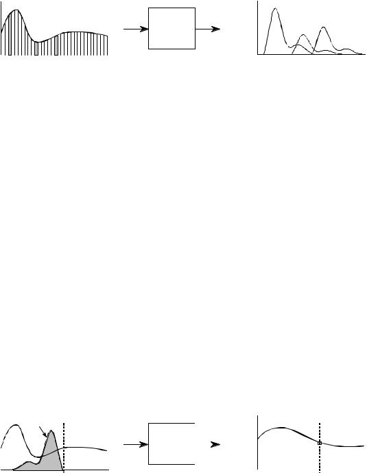
Figure 13-2 shows how convolution is viewed from the input side. An input signal, x (t), is passed through a system characterized by an impulse response, h (t), to produce an output signal, y (t). This can be written in the familiar mathematical equation, y (t) ' x (t) th (t). The input signal is divided into narrow columns, each short enough to act as an impulse to the system. In other words, the input signal is decomposed into an infinite number of scaled and shifted delta functions. Each of these impulses produces a scaled and shifted version of the impulse response in the output signal. The final output signal is then equal to the combined effect, i.e., the sum of all of the individual responses.
For this scheme to work, the width of the columns must be much shorter than the response of the system. Of course, mathematicians take this to the extreme by making the input segments infinitesimally narrow, turning the situation into a calculus problem. In this manner, the input viewpoint describes how a single point (or narrow region) in the input signal affects a larger portion of output signal.
In comparison, the output viewpoint examines how a single point in the output signal is determined by the various values from the input signal. Just as with discrete signals, each instantaneous value in the output signal is affected by a section of the input signal, weighted by the impulse response flipped left-for-right. In the discrete case, the signals are multiplied and summed. In the continuous case, the signals are multiplied and integrated. In equation form:
EQUATION 13-1 |
|
%4 |
|
|
y (t ) ' |
m |
x (J) h (t & J) d J |
||
The convolution integral. This equation |
||||
defines the meaning of: y (t ) ' x (t )th (t ). |
|
|
||
|
|
&4 |
|
This equation is called the convolution integral, and is the twin of the convolution sum (Eq. 6-1) used with discrete signals. Figure 13-3 shows how this equation can be understood. The goal is to find an expression for calculating the value of the output signal at an arbitrary time, t. The first step is to change the independent variable used to move through the input signal and the impulse response. That is, we replace t with J (a lower case
Chapter 13Continuous Signal Processing |
247 |
|
a |
|
|
a |
|
|
|
|
|
|
|
x(t) |
c |
Linear |
y(t) |
b |
c |
|
System |
|
|
||
|
b |
|
|
||
|
time (t) |
|
|
time(t) |
|
FIGURE 13-2
Convolution viewed from the input side. The input signal, x(t) , is divided into narrow segments, each acting as an impulse to the system. The output signal, y (t), is the sum of the resulting scaled and shifted impulse responses. This illustration shows how three points in the input signal contribute to the output signal.
Greek tau). This makes x (t) and h (t) become x (J)and h (J), respectively. This change of variable names is needed because t is already being used to represent the point in the output signal being calculated. The next step is to flip the impulse response left-for-right, turning it into h (& J). Shifting the flipped impulse response to the location t, results in the expression becoming h(t& J) . The input signal is then weighted by the flipped and shifted impulse response by multiplying the two, i.e., x (J) h (t& J) . The value of the output signal is then found by integrating this weighted input signal from negative to positive infinity, as described by Eq. 13-1.
If you have trouble understanding how this works, go back and review the same concepts for discrete signals in Chapter 6. Figure 13-3 is just another way of describing the convolution machine in Fig. 6-8. The only difference is that integrals are being used instead of summations. Treat this as an extension of what you already know, not something new.
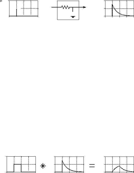
An example will illustrate how continuous convolution is used in real world problems and the mathematics required. Figure 13-4 shows a simple continuous linear system: an electronic low-pass filter composed of a single resistor and a single capacitor. As shown in the figure, an impulse entering this system produces an output that quickly jumps to some value, and then exponentially decays toward zero. In other words, the impulse response of this simple electronic circuit is a one-sided exponential. Mathematically, the
h(t-J) t
x(J)  x(J)
x(J)
|
|
|
t |
|
Linear |
|
y(t) |
|
? |
System |
|
|
|
|
time (J) |
time(t) |
FIGURE 13-3
Convolution viewed from the output side. Each value in the output signal is influenced by many points from the input signal. In this figure, the output signal at time t is being calculated. The input signal, x (J), is weighted (multiplied) by the flipped and shifted impulse response, given by h ( t&J) . Integrating the weighted input signal produces the value of the output point, y (t)
248 |
The Scientist and Engineer's Guide to Digital Signal Processing |
|
|
*(t) |
h(t) |
Amplitude
2
1 


0 


 -1 0 1 2 3
Time
R
C 
2
Amplitude |
1 |
|
|
|
|
|
|
|
|
|
|
|
0 |
|
|
|
|
|
-1 |
0 |
1 |
2 |
3 |
Time
FIGURE 13-4
Example of a continuous linear system. This electronic circuit is a low-pass filter composed of a single resistor and capacitor. The impulse response of this system is a one-sided exponential.
impulse response of this system is broken into two sections, each represented by an equation:
h (t ) |
' |
0 |
for t < 0 |
h (t ) |
' |
"e &" t |
for t $ 0 |
where " ' 1/RC (R is in ohms, C is in farads, and t is in seconds). Just as in the discrete case, the continuous impulse response contains complete information about the system, that is, how it will react to all possible signals. To pursue this example further, Fig. 13-5 shows a square pulse entering the system, mathematically expressed by:
x (t ) |
' |
1 |
for 0 # t # 1 |
x (t ) |
' |
0 |
otherwise |
Since both the input signal and the impulse response are completely known as mathematical expressions, the output signal, y (t), can be calculated by evaluating the convolution integral of Eq. 13-1. This is complicated by the fact that both signals are defined by regions rather than a single


 Amplitude
x(t)
2
1 


0 

 -1 0 1 2 3
Time
Amplitude
|
|
h(t) |
|
|
|
|
|
y(t) |
|
|
2 |
|
|
|
|
Amplitude |
2 |
|
|
|
|
1 |
|
|
|
|
1 |
|
|
|
|
|
|
|
|
|
|
|
|
|
|
||
0 |
|
|
|
|
|
0 |
|
|
|
|
-1 |
0 |
1 |
2 |
3 |
|
-1 |
0 |
1 |
2 |
3 |
|
|
Time |
|
|
|
|
|
Time |
|
|
FIGURE 13-5
Example of continuous convolution. This figure illustrates a square pulse entering an RC low-pass filter (Fig. 13-4). The square pulse is convolved with the system's impulse response to produce the output.
|
|
Chapter 13Continuous Signal Processing |
249 |
||||||||
a. No overlap |
|
|
b. Partial overlap |
c. Full overlap |
|
|
|||||
(t < 0) |
|
|
|
(0 # t # 1) |
|
(t > 1) |
|
|
|||
t |
|
|
|
|
|
t |
|
|
t |
||
|
|
|
|
||||||||
|
|
|
|
|
|
|
|
|
|
|
|
|
|
|
|
|
|
|
|
|
|
|
|
0 |
1 |
0 |
1 |
0 |
1 |
J |
|
J |
|
J |
|
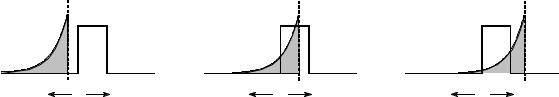
FIGURE 13-6
Calculating a convolution by segments. Since many continuous signals are defined by regions, the convolution calculation must be performed region-by-region. In this example, calculation of the output signal is broken into three sections: (a) no overlap, (b) partial overlap, and (c) total overlap, of the input signal and the shiftedflipped impulse response.
mathematical expression. This is very common in continuous signal processing. It is usually essential to draw a picture of how the two signals shift over each other for various values of t. In this example, Fig. 13-6a shows that the two signals do not overlap at all for t < 0 . This means that the product of the two signals is zero at all locations along the J axis, and the resulting output signal is:
y (t ) ' 0
for t < 0
A second case is illustrated in (b), where t is between 0 and 1. Here the two signals partially overlap, resulting in their product having nonzero values between J ' 0 and J ' t . Since this is the only nonzero region, it is the only section where the integral needs to be evaluated. This provides the output signal for 0 # t #1 , given by:
4
y (t ) |
' m x (J) h (t & J) d J |
(start with Eq. 13-1) |
|
& 4 |
|
|
t |
|
y (t ) |
' m1@ "e & "( t& J) d J |
(plug in the signals) |
|
0 |
|
|
t |
|
y (t ) ' e
y (t ) ' e
& "t |
[ e |
"J |
] / |
(evaluate the integral) |
|
|
|
||
|
|
|
0 |
|
& "t |
[ e "t |
& 1 ] |
(reduce) |
|
y (t ) ' 1 & e & "t |
for 0 # t # 1 |
250 |
The Scientist and Engineer's Guide to Digital Signal Processing |
Figure (c) shows the calculation for the third section of the output signal, where t > 1. Here the overlap occurs between J ' 0 and J ' 1 , making the calculation the same as for the second segment, except a change to the limits of integration:
|
|
1 |
|
|
|
|
|
y (t ) |
' m1@ "e & "( t& J) d J |
(plug into Eq. 13-1) |
|||||
|
|
0 |
|
|
|
|
|
|
|
|
|
|
|
1 |
|
y (t ) |
' |
e |
& "t |
[ e |
"J |
] / |
(evaluate the integral) |
|
|
||||||
|
|
|
|
|
|
0 |
|
y (t ) |
' [ e "& 1 ] e & "t |
for t > 1 |
|||||
The waveform in each of these three segments should agree with your knowledge of electronics: (1) The output signal must be zero until the input signal becomes nonzero. That is, the first segment is given by y (t ) ' 0 for t < 0 . (2) When the step occurs, the RC circuit exponentially increases to match the input, according to the equation: y (t ) ' 1 & e & " t . (3) When the input is returned to zero, the output exponentially decays toward zero, given by the equation: y (t ) ' ke & " t (where k ' e "& 1 , the voltage on the capacitor just before the discharge was started).
More intricate waveforms can be handled in the same way, although the mathematical complexity can rapidly become unmanageable. When faced with a nasty continuous convolution problem, you need to spend significant time evaluating strategies for solving the problem. If you start blindly evaluating integrals you are likely to end up with a mathematical mess. A common strategy is to break one of the signals into simpler additive components that can be individually convolved. Using the principles of linearity, the resulting waveforms can be added to find the answer to the original problem.
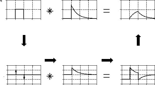
Figure 13-7 shows another strategy: modify one of the signals in some linear way, perform the convolution, and then undo the original modification. In this example the modification is the derivative, and it is undone by taking the integral. The derivative of a unit amplitude square pulse is two impulses, the first with an area of one, and the second with an area of negative one. To understand this, think about the opposite process of taking the integral of the two impulses. As you integrate past the first impulse, the integral rapidly increases from zero to one, i.e., a step function. After passing the negative impulse, the integral of the signal rapidly returns from one back to zero, completing the square pulse.
Taking the derivative simplifies this problem because convolution is easy when one of the signals is composed of impulses. Each of the two impulses in x )(t ) contributes a scaled and shifted version of the impulse response to
Chapter 13Continuous Signal Processing |
251 |
x(t)
2
Amplitude |
1 |
|
|
|
|
|
|
|
|
|
|
|
0 |
|
|
|
|
|
-1 |
0 |
1 |
2 |
3 |
Time
|
|
|
h(t) |
|
|
|
|
|
y(t) |
|
|
Amplitude |
2 |
|
|
|
|
Amplitude |
2 |
|
|
|
|
1 |
|
|
|
|
1 |
|
|
|
|
||
|
|
|
|
|
|
|
|
|
|
||
|
0 |
|
|
|
|
|
0 |
|
|
|
|
|
-1 |
0 |
1 |
2 |
3 |
|
-1 |
0 |
1 |
2 |
3 |
|
|
|
Time |
|
|
|
|
|
Time |
|
|
d/dt
|
|
xN(t) |
|
|
|
|
h(t) |
|
|
2 |
|
|
|
|
2 |
|
|
|
|
1 |
|
|
|
|
1 |
|
|
|
|
Amplitude -1 |
|
|
|
|
Amplitude-1 |
|
|
|
|
0 |
|
|
|
|
0 |
|
|
|
|
-2 |
|
|
|
|
-2 |
|
|
|
|
-1 |
0 |
1 |
2 |
3 |
-1 |
0 |
1 |
2 |
3 |
|
|
Time |
|
|
|
|
Time |
|
|
|
|
I |
|
|
|
|
yN(t) |
|
|
2 |
|
|
|
|
1 |
|
|
|
|
Amplitude-1 |
|
|
|
|
0 |
|
|
|
|
-2 |
|
|
|
|
-1 |
0 |
1 |
2 |
3 |
|
|
Time |
|
|
FIGURE 13-7
A strategy for convolving signals. Convolution problems can often be simplified by clever use of the rules governing linear systems. In this example, the convolution of two signals is simplified by taking the derivative of one of them. After performing the convolution, the derivative is undone by taking the integral.
the derivative of the output signal, y )(t). That is, by inspection it is known that: y )(t ) ' h (t ) & h (t& 1). The output signal, y (t ) , can then be found by plugging in the exact equation for h (t ) , and integrating the expression.
A slight nuisance in this procedure is that the DC value of the input signal is lost when the derivative is taken. This can result in an error in the DC value of the calculated output signal. The mathematics reflects this as the arbitrary constant that can be added during the integration. There is no systematic way of identifying this error, but it can usually be corrected by inspection of the problem. For instance, there is no DC error in the example of Fig. 13-7. This is known because the calculated output signal has the correct DC value when t becomes very large. If an error is present in a particular problem, an appropriate DC term is manually added to the output signal to complete the calculation.
This method also works for signals that can be reduced to impulses by taking the derivative multiple times. In the jargon of the field, these signals are called piecewise polynomials. After the convolution, the initial operation of multiple derivatives is undone by taking multiple integrals. The only catch is that the lost DC value must be found at each stage by finding the correct constant of integration.

252 |
The Scientist and Engineer's Guide to Digital Signal Processing |
Before starting a difficult continuous convolution problem, there is another approach that you should consider. Ask yourself the question: Is a mathematical expression really needed for the output signal, or is a graph of the waveform sufficient? If a graph is adequate, you may be better off to handle the problem with discrete techniques. That is, approximate the continuous signals by samples that can be directly convolved by a computer program. While not as mathematically pure, it can be much easier.
The Fourier Transform
The Fourier Transform for continuous signals is divided into two categories, one for signals that are periodic, and one for signals that are aperiodic. Periodic signals use a version of the Fourier Transform called the Fourier Series, and are discussed in the next section. The Fourier Transform used with aperiodic signals is simply called the Fourier Transform. This chapter describes these Fourier techniques using only real mathematics, just as the last several chapters have done for discrete signals. The more powerful use of complex mathematics will be reserved for Chapter 31.
Figure 13-8 shows an example of a continuous aperiodic signal and its frequency spectrum. The time domain signal extends from negative infinity to positive infinity, while each of the frequency domain signals extends from zero to positive infinity. This frequency spectrum is shown in rectangular form (real and imaginary parts); however, the polar form (magnitude and phase) is also used with continuous signals. Just as in the discrete case, the synthesis equation describes a recipe for constructing the time domain signal using the data in the frequency domain. In mathematical form:
|
% 4 |
|
|
x (t ) ' |
1 |
m Re X (T) cos (Tt ) |
& Im X (T) sin(Tt ) d T |
B |
|||
|
0 |
|
|
EQUATION 13-2
The Fourier transform synthesis equation. In this equation, x(t) is the time domain signal being synthesized, and Re X(T) & Im X(T) are the real and imaginary parts of the frequency spectrum, respectively.
In words, the time domain signal is formed by adding (with the use of an integral) an infinite number of scaled sine and cosine waves. The real part of the frequency domain consists of the scaling factors for the cosine waves, while the imaginary part consists of the scaling factors for the sine waves. Just as with discrete signals, the synthesis equation is usually written with negative sine waves. Although the negative sign has no significance in this discussion, it is necessary to make the notation compatible with the complex mathematics described in Chapter 29. The key point to remember is that some authors put this negative sign in the equation, while others do not. Also notice that frequency is represented by the symbol, T, a lower case