Beginning Algorithms (2006)

Chapter 7

Now things get interesting. The algorithm proceeds as before, with the left index advancing until it finds an item larger than the partitioning item, in this case the letter T. The right index then advances to the left but stops when it reaches the same value as the left index. There is no advantage to going beyond this point, as all items to the left of this index have been dealt with already. The list is now in the state shown in Figure 7-23, with both left and right indexes pointing at the letter T.

F A I C K E G I T R S O R S U T Q U N

Figure 7-23: The left and right indexes meet at the partitioning position.

The point where the two indexes meet is the partitioning position — that is, it is the place in the list where the partitioning value actually belongs. Therefore, you do one final swap between this location and the partitioning value at the far right of the list to move the partitioning value into its final sorted position. When this is done, the letter N is in the partitioning position, with all of the values to its left being smaller, and all of the values to its right being larger (see Figure 7-24).

Less than ‘N’ Greater than ‘N’

F A I C K E G I N R S O R S U T Q U T

Figure 7-24: The partitioning item in final sorted position.

All the steps illustrated so far have resulted in only the letter N being in its final sorted position. The list itself is far from sorted. However, the list has been divided into two parts that can be sorted independently of each other. You simply sort the left part of the list, and then the right part of the list, and the whole list is sorted. This is where the recursion comes in. You apply the same quicksort algorithm to each of the two sublists to the left and right of the partitioning item.

You have two cases to consider when building recursive algorithms: the base case and the general case. For quicksort, the base case occurs when the sublist to be sorted has only one element; it is by definition already sorted and nothing needs to be done. The general case occurs when there is more than one item, in which case you apply the preceding algorithm to partition the list into smaller sublists after placing the partitioning item into the final sorted position.

Having seen an example of how the quicksort algorithm works, you can test it in the next Try It Out exercise.

154

Advanced Sorting

You start by creating a test case that is specific to the quicksort algorithm:

package com.wrox.algorithms.sorting;

public class QuicksortListSorterTest extends AbstractListSorterTest { protected ListSorter createListSorter(Comparator comparator) {

return new QuicksortListSorter(comparator);

}

}

How It Works

The preceding test extends the general-purpose test for sorting algorithms that you created in Chapter 6. All you need to do to test the quicksort implementation is instantiate it by overriding the createListSorter() method.

In the next Try It Out, you implement quicksort.

First you create the QuicksortListSorter, which will be familiar to you because its basic structure is very similar to the other sorting algorithms you have seen so far. It implements the ListSorter interface and accepts a comparator that imposes the sorted order on the objects to be sorted:

package com.wrox.algorithms.sorting;

import com.wrox.algorithms.lists.List;

public class QuicksortListSorter implements ListSorter { private final Comparator _comparator;

public QuicksortListSorter(Comparator comparator) {

assert comparator != null : “comparator cannot be null”; _comparator = comparator;

}

...

}

You use the sort() method to delegate to the quicksort() method, passing in the indexes of the first and last elements to be sorted. In this case, this represents the entire list. This method will later be called recursively, passing in smaller sublists defined by different indexes.

public List sort(List list) {

assert list != null : “list cannot be null”;

quicksort(list, 0, list.size() - 1);

return list;

}

155

Chapter 7

You implement the quicksort by using the indexes provided to partition the list around the partitioning value at the end of the list, and then recursively calling quicksort() for both the left and right sublists:

private void quicksort(List list, int startIndex, int endIndex) { if (startIndex < 0 || endIndex >= list.size()) {

return;

}

if (endIndex <= startIndex) { return;

}

Object value = list.get(endIndex);

int partition = partition(list, value, startIndex, endIndex - 1); if (_comparator.compare(list.get(partition), value) < 0) {

++partition;

}

swap(list, partition, endIndex);

quicksort(list, startIndex, partition - 1); quicksort(list, partition + 1, endIndex);

}

You use the partition() method to perform the part of the algorithm whereby out-of-place items are swapped with each other so that small items end up to the left, and large items end up to the right:

private int partition(List list, Object value, int leftIndex, int rightIndex) { int left = leftIndex;

int right = rightIndex;

while (left < right) {

if (_comparator.compare(list.get(left), value) < 0) { ++left;

continue;

}

if (_comparator.compare(list.get(right), value) >= 0) { --right;

continue;

}

swap(list, left, right); ++left;

}

return left;

}

156

Advanced Sorting

Finally, you implement a simple swap() method that protects itself against calls to swap an item with itself:

private void swap(List list, int left, int right) { if (left == right) {

return;

}

Object temp = list.get(left); list.set(left, list.get(right)); list.set(right, temp);

}

How It Works

The quicksort() method begins by bounds-checking the two indexes it is passed. This enables later code to be simplified by ignoring this concern. It next obtains the partitioning value from the far right end of the list. The next step is to obtain the partitioning position by delegating to the partition() method.

The partition() method contains a test to check whether the value at the partitioning location is smaller than the partitioning value itself. This can happen, for example, when the partitioning value is the largest value in the whole list of items. Given that you are choosing it at random, this can happen very easily. In this case, you advance the partitioning index by one position. This code is written such that the left and right indexes always end up with the same value, as they did in the explanation of the algorithm earlier in the chapter. The value at this index is the return value from this method.

Understanding the Compound Comparator

and Stability

Before considering the third advanced sorting algorithm, this section elaborates on the discussion of stability, which was first brought to your attention in the previous chapter. Now is a good time because the two algorithms discussed so far in this chapter share the shortcoming that they are not stable. The algorithm covered next — mergesort — is stable, so now is a good opportunity to deal with the lack of stability in shellsort and quicksort.

As you learned in Chapter 6, stability is the tendency of a sorting algorithm to maintain the relative position of items with the same sort key during the sort process. Quicksort and shellsort lack stability, as they pay no attention at all to the items that are near each other in the original input list. This section discusses a way to compensate for this issue when using one of these algorithms: the compound comparator.

The example in Chapter 6 was based on a list of people that was sorted by either first name or last name. The relative order of people with the same last name is maintained (that is, they were ordered by first name within the same last name group) if the algorithm used is stable. Another way to achieve the same effect is to use a compound key for the person object, consisting of both the first name and last name when sorting by first name, and both the last name and first name when sorting by last name. As you saw in Chapter 6, it is often possible to create useful general-purpose comparators to solve many different problems. That is the approach taken in the next Try It Out, where you create a compound comparator that can wrap any number of standard single-value comparators to achieve a sort outcome based on a compound key.

157

Chapter 7

The tests for the compound comparator need the services of a dummy comparator that always returns a known value from its compare() method. Give this the obvious name of FixedComparator. The code is shown here:

package com.wrox.algorithms.sorting;

public class FixedComparator implements Comparator { private final int _result;

public FixedComparator(int result) { _result = result;

}

public int compare(Object left, Object right) { return _result;

}

}

You can now begin writing tests for the compound comparator. You have to cover three basic cases: it returns zero, it returns a positive integer, or it returns a negative integer from its compare() method. Each of these tests adds multiple fixed comparators to the compound comparator. The first of these is set up to return zero, indicating that the compound comparator must use more than the first element of the compound key to sort the items. The code for the three test cases is shown here:

package com.wrox.algorithms.sorting;

import junit.framework.TestCase;

public class CompoundComparatorTest extends TestCase { public void testComparisonContinuesWhileEqual() {

CompoundComparator comparator = new CompoundComparator(); comparator.addComparator(new FixedComparator(0)); comparator.addComparator(new FixedComparator(0)); comparator.addComparator(new FixedComparator(0));

assertTrue(comparator.compare(“IGNORED”, “IGNORED”) == 0);

}

public void testComparisonStopsWhenLessThan() { CompoundComparator comparator = new CompoundComparator(); comparator.addComparator(new FixedComparator(0)); comparator.addComparator(new FixedComparator(0)); comparator.addComparator(new FixedComparator(-57)); comparator.addComparator(new FixedComparator(91));

assertTrue(comparator.compare(“IGNORED”, “IGNORED”) < 0);

}

public void testComparisonStopsWhenGreaterThan() { CompoundComparator comparator = new CompoundComparator();

158

Advanced Sorting

comparator.addComparator(new FixedComparator(0)); comparator.addComparator(new FixedComparator(0)); comparator.addComparator(new FixedComparator(91)); comparator.addComparator(new FixedComparator(-57));

assertTrue(comparator.compare(“IGNORED”, “IGNORED”) > 0);

}

}

How It Works

The test relies upon being able to add any number of other comparators to the new CompoundComparator in sequence. The first test adds four comparators that all return zero when their respective compare() methods are called. The idea is that the CompoundComparator checks with each of its nested comparators in turn, returning as soon as one of them returns a nonzero value. If all of the nested comparators return zero, the overall comparison has determined that the objects are the same.

The second test sets up a series of nested comparators whereby the third one returns a negative value. The intended behavior of the CompoundComparator is that it should return the first nonzero value from its nested comparators. The test asserts that this behavior is correct. The final test does the same job but with a positive return value.

In the next Try It Out, you implement CompoundComparator.

You start by creating the class to implement the Comparator interface, and give it a private List in which to hold the unknown number of comparators for each element of the compound sort key:

package com.wrox.algorithms.sorting;

import com.wrox.algorithms.iteration.Iterator; import com.wrox.algorithms.lists.ArrayList; import com.wrox.algorithms.lists.List;

public class CompoundComparator implements Comparator { private final List _comparators = new ArrayList();

...

}

You provide the addComparator() method to allow any number of comparators to be wrapped by the compound comparator:

public void addComparator(Comparator comparator) {

assert comparator != null : “comparator can’t be null”; assert comparator != this : “can’t add comparator to itself”;

_comparators.add(comparator);

}

159

Chapter 7

Finally, implement compare() to use each of the wrapped comparators in turn, returning as soon as one of them returns a nonzero result:

public int compare(Object left, Object right) { int result = 0;

Iterator i = _comparators.iterator();

for (i.first(); !i.isDone(); i.next()) {

result = ((Comparator) i.current()).compare(left, right); if (result != 0) {

break;

}

}

return result;

}

The CompoundComparator is extremely useful because it can re-use any existing comparators to overcome a lack of stability, or simply to sort on a compound key.

Understanding the Mergesor t Algorithm

Mergesort is the last of the advanced sorting algorithms covered in this chapter. Like quicksort, it is possible to implement mergesort both recursively and iteratively, but we implement it recursively in this section. Unlike quicksort, mergesort does not sort the list it is provided in place; rather, it creates a new output list containing the objects from the input list in sorted order.

Merging

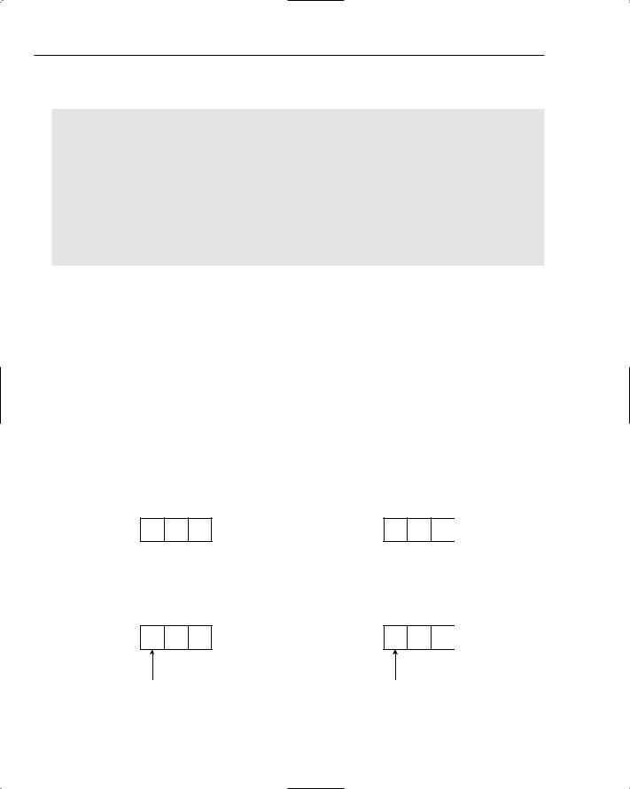
Mergesort is built upon the concept of merging. Merging takes two (already sorted) lists and produces a new output list containing all of the items from both lists in sorted order. For example, Figure 7-25 shows two input lists that need to be merged. Note that both lists are already in sorted order.

Figure 7-25: Two already sorted lists that we want to merge.

The process of merging begins by placing indexes at the head of each list. These will obviously point to the smallest items in each list, as shown in Figure 7-26.

Figure 7-26: Merging begins at the head of each list.

160

Advanced Sorting

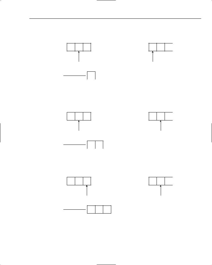
The items at the start of each list are compared, and the smallest of them is added to the output list. The next item in the list from which the smallest item was copied is considered. The situation after the first item has been moved to the output list is shown in Figure 7-27.

OUTPUT

A

Figure 7-27: The first item is added to the output list.

The current items from each list are compared again, with the smallest being placed on the output list. In this case, it’s the letter D from the second list. Figure 7-28 shows the situation after this step has taken place.

OUTPUT

A D

Figure 7-28: The second item is added to the output list.

The process continues; this time the letter F from the first list is the smaller item and it is copied to the output list, as shown in Figure 7-29.

OUTPUT

A D F

Figure 7-29: The third item is placed on the output list.

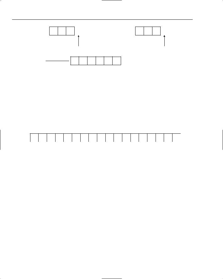
This process continues until both input lists have been exhausted and the output contains each item from both lists in sorted order. The final state is shown in Figure 7-30.

161

Chapter 7

OUTPUT

A D F G L M

Figure 7-30: The completed merge process.

The mergesort Algorithm

The mergesort algorithm is based upon the idea of merging. As with the quicksort algorithm, you approach mergesort with recursion, but quicksort was a divide-and-conquer approach, whereas the mergesort algorithm describes more of a combine-and-conquer technique. Sorting happens at the top level of the recursion only after it is complete at all lower levels. Contrast this with quicksort, where one item is placed into final sorted position at the top level before the problem is broken down and each recursive call places one further item into sorted position.

This example uses the list of letters shown in Figure 7-31 as the sample data.

R E C U R S I V E M E R G E S O R T

Figure 7-31: Sample list to demonstrate recursive mergesort.

Like all the sorting algorithms, mergesort is built upon an intriguingly simple idea. Mergesort simply divides the list to be sorted in half, sorts each half independently, and merges the result. It sounds almost too simple to be effective, but it will still take some explaining. Figure 7-32 shows the sample list after it has been split in half. When these halves are sorted independently, the final step will be to merge them together, as described in the preceding section on merging.

Figure 7-32: The sample list when split in half.

A key difference between mergesort and quicksort is that the way in which the list is split in mergesort is completely independent of the input data itself. Mergesort simply halves the list, whereas quicksort partitions the list based on a chosen value, which can split the list at any point on any pass.

So how do you sort the first half of the list? By applying mergesort again! You split that half in half, sort each half independently, and merge them. Figure 7-33 shows half of the original list split in half itself.

162

Figure 7-33: The first recursive call to mergesort the first half of the original list.

How do you sort the first half of the first half of the original list? Another recursive call to mergesort, of course. By now you will no doubt be getting the idea that you keep recursing until you reach a sublist with a single item in it, which of course is already sorted like any single-item list, and that will be the base case for this recursive algorithm. You saw the general case already — that is, when there is more than one item in the list to be sorted, split the list in half, sort the halves, and then merge them together.

Figure 7-34 shows the situation at the third level of recursion.

Figure 7-34: Third level of recursion during mergesort.

As you still have not reached a sublist with one item in it, you continue the recursion to yet another level, as shown in Figure 7-35.

Figure 7-35: Fourth level of recursion during mergesort.

At the level of recursion shown in Figure 7-35, you are trying to sort the two-element sublist containing the letters R and E. This sublist has more than one item in it, so once more you need to split and sort the halves as shown in Figure 7-36.

163