Chau Chemometrics From Basics to Wavelet Transform

tendency to combine different chemical devices together to form ‘‘hyphenated instruments’’ for multidimensional measurements. These modern analytical instruments produce multidimensional data that give more information on the analytes. However, this demands larger storage capacities for the instruments, especially when libraries or databases are used for matching, such as infrared (IR) spectroscopy, mass spectroscopy (MS), and nuclear magnetic resonance (NMR) spectroscopy. An alternative to reduce the storage space and the processing time is through signal compression.

In order to store chemical data efficiently, the compression method must not be too computationally demanding. Furthermore, the discrepancy between the original dataset and the data reconstructed from the compressed form should be reasonably small.

Different methods for chemical signal compression have been proposed in the literature and can be classified into two categories. The first one lowers the resolution of the original signal by reducing the number of data to be retained, such as the binary coding method and factor analysis. The second type retains the resolution of the signal through transformation of the signal from one form to another one, such as the well-known FT method. In spite of the availability of these methods, the application of WT on compressing analytical data was proposed and the method was proved to be very efficient.

5.1.1. Principle and Algorithm

In signal processing of chemical datasets, fast wavelet transform (FWT) is usually employed. The algorithm of FWT has been described in the Chapter 4. For a signal c0, its FWT can be implemented by

N

where c and d with the index represent the elements of the decomposed components c and d from the original signal c0 by WT, H = {h−k }k Z and

ψ(x ) and the scaling function φ(x ), and N represents the length of the vector cj −1. In these two equations, the WT of the signal c0 means that the resulting signals c1 (called discrete approximation or scale coefficient ) and d1 (called discrete detail or wavelet coefficient ) are, respectively, the convolution of c0 with the discrete filters H and G followed by the property of ‘‘downsampling by factor 2.’’

A schematic diagram showing the operation of the FWT method is shown in Figure 5.1. When FWT is applied to a signal c0 = {c0,0, c0,1, . . . , c0,N−1} with length N( = 2P ) and P is any positive integer, the scale coefficients cj and wavelet coefficients dj at resolution level j are determined by Equations (5.1) and (5.2), respectively. For resolution level j = 1, the numbers of the elements of c1 and d1 are the same and equal to N/2. Then, the decomposition process is applied to c1 again to obtain the coefficients at the next resolution level. The process is repeated until the desired J th resolution level is reached. Finally, the original signal is expressed as a collection of the scale and wavelet coefficients in the form of {cJ , dJ , dJ −1, . . . , d1}. The total number of coefficients equals the length of the original signal. Because of the downsampling property of the algorithm, it is called the ‘‘tree algorithm’’ or ‘‘pyramid algorithm.’’

The original signal c0 can be reconstructed from the scale coefficients cj and wavelet coefficients dj , j = J , . . . , 1, following the backward procedures of Figure 5.1 using the inverse fast wavelet transform (IFWT)

Figure 5.1. A schematic diagram showing the operation of the FWT method on a signal with data length of N = 1024.

where H and G are conjugate filters of the filters H and G . In the calculation, cj and dj must followed by a ‘‘upsampling by factor 2’’ with zeros added between each adjacent elements of the vectors.

The decomposition and reconstruction equations presented above are useful for data compression because the WT procedure is capable of retaining a large percentage of the total energy of the signal in the scale coefficients cj at different resolution levels. Since the wavelet coefficients are generated from the highpass filter G , dj reflects the high-frequency information contained in the original data set at the j th level. For most analytical signals, the high-frequency components are usually considered as noise and disposable. Hence, only a small number of the wavelet coefficients is needed to effectively represent the original signal.

For determining which coefficients should be retained, the thresholding method is generally used. Since only the larger coefficients are considered to represent useful information, those coefficients with absolute values greater than a given threshold ε are retained. It is obvious that the choice of the threshold ε affects the compression efficiency and the quality of the reconstructed signal. Usually, a larger ε gives a higher compression ratio but a poorer reconstructed signal. Different procedures for the thresholding operation and the determination of the threshold are discussed in Section 5.1.3.

The general procedure of data compression using WT can be outlined as follows:

1.Apply a WT treatment to the original signal c0 and to obtain the vector of the scale and wavelet coefficients w = {cJ , dJ , dJ −1, . . . , d1} using Equations (5.1) and (5.2).

2.Suppress the small coefficients in w that are considered too small to contain the useful information of the signal using the thresholding methods. The number of wavelet coefficients to be stored will be decided by the value of the threshold ε.

3.Store the suppressed vector wstore as the compressed result.

4.Reconstruct the original signal by applying the inverse transform to the wstore using Equation (5.5) when an original signal is needed.

Example 5.1 illustrates the operation of the above mentioned data compression procedure.

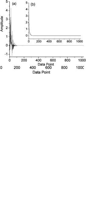
Example 5.1: Compression of a Simulated Signal Using FWT. Figure 5.2, curve (a) shows a simulated signal denoted as a row vector c0

Figure 5.2. Plot of a simulated signal with 1024 data points (a) and the reconstructed signal by WT using 128 coefficients (b).

with 1024 data points. The WT is applied to c0 with the Daubechies18 (L = 18, where L represents the length of the wavelet filters H and G) filters and resolution level J = 4, we can obtain the coefficients vector w shown in Figure 5.3, plot (a). The vector is in the order of {c4,(1,... ,64),

d4,(65,... ,128), d3,(129,... ,256), d2,(253,... ,512), d1,(513,... ,1024)}. It is clearer in Figure

5.3, plot (b), which is plotted by the absolute values of these coefficients sorted by their magnitudes. It should be noted that WT with different filter and different resolution level J will give a different result; this is discussed

Figure 5.3. Plot of the coefficient vector obtained by applying WT to the simulated signal (a) and its absolute values sorted by magnitude (b).

further in Section 5.1.4. From Figure 5.3, it can be seen that most of the coefficients are small enough to be neglected. The original signal can be represented by only a few WT coefficients.

In order to suppress the small coefficients in w, a proper value of the threshold ε is required. In this example, a threshold for retaining 128 coefficients was adopted; that is, only 128 largest coefficients was retained while all other coefficients were set to have value zero. In this way, the compression ratio is 1024/128=8.

Figure 5.2, curve (b) shows the reconstructed signal yˆi from the 128 retained coefficients as obtained from Example 5.1. Comparing with the original signal yi in Figure 5.2, curve (a), it can be seen that there is almost no difference between them. The root-mean-square (RMS) error

as calculated by N (yˆ − y )2/N is only 2.8587 × 10−5.

i =1 i i

Computational Details of Example 5.1

1.Generate the original signal with 1024 data points; refer to curve

(a) of Figure 5.2 using the Gaussian equation.

2.Make a wavelet filter---Daubechies18.

3.Set resolution level J = 4 (10 − 6).

4.Perform forward WT to obtain the wavelet coefficients.

5.Perform hard thresholding to the wavelet coefficients keeping the 128 largest coefficients.

6.Construct the signal by applying inverse WT to the 128 retained coefficients.

7.Display Figure 5.2, curves (a) and (b).

8.Display Figure 5.3, plots (a) and (b).

9.Display the RMS error between the original signal and the reconstructed signal.

Note: The MATLAB codes of the examples presented in this chapter are available at the ftp (File Transfer Protocol) server of the publisher (ftp://www.wiley.com/chemistry), or by sending an email to the author (xshao@ustc.edu.cn).

Most of the programs were developed based on the WaveLab 7.0. The WaveLab is a toolbox developed by the WaveLab Development Team (Jonathan Buckheit, Shaobing Chen, David Donoho, Iain Johnstone, and Jeffrey Scargle) at Stanford University, and it can be downloaded from http://www-stat.stanford.edu/ wavelab/. Instructions for installation are also available from the Website. You must install the WaveLab before running these programs.

154 application of wavelet transform in chemistry

In the preceding FWT calculation, the length of the original signal must be equal to 2P . If an odd-number dataset is encountered at a particular resolution level, FWT calculation will be stopped automatically and cannot be processed to the next resolution level. However, in practice, the length of a chemical signal depends on the sampling time (for chromatograms) or wavelength range (for spectra). It is not easy for a chemical instrument to generate 2P data exactly.

Several methods can be used to cope with the problem, such as the zero padding, symmetrization, extrapolation, and periodization, which have been introduced in Chapter 4. Besides, truncation of data at one or both ends of the original data to the previous power of 2 can also be adopted in some cases. Although these methods are widely used, new ones have also been proposed to improve the FWT algorithm. One of these new methods is called the coefficient position-retaining (CPR) method and is described below.

A schematic diagram for applying FWT to a signal with 1231 data with the use of CPR is shown in Figure 5.4. In the CPR approach, if the data length of a scale coefficients cj at resolution level j , NC,j , is an even number, the FWT is applied as usual via Equations (5.1) and (5.2). The scale and wavelet coefficients obtained at resolution ( j +1) will have the same length, which is equal to NC,j /2. On the other hand, if NC,j is an odd number, FWT is adopted without using the last coefficient of cj in the calculation. This coefficient is retained and transferred downward to the same position at the next resolution level. It becomes the last coefficient of dj +1 at resolution level ( j +1). As a result, the scale and wavelet coefficients will have (NC,j − 1)/2 and (NC,j − 1)/2 + 1 elements, respectively.

Figure 5.4. A schematic diagram showing the operation of FWT coupled with CPR on a signal with data length of N = 1231.

The calculation of the WPT decomposition can be implemented using equations similar to Equations (5.1)--(5.4) with

where p = 0, . . . , 2 j −1 −1. Signal reconstruction can also be implemented using equations similar to Equations (5.7) and (5.8) as

In this manner, data compression using WPT involves the following procedures:

1.Apply WPT to the original signal w00 up to level J and to obtain all the coefficients wjp for j = 1, . . . , J and p = 0, . . . , 2 j −1 − 1 using Equations (5.7) and (5.8).

2.Find the best basis to express the original signal.

3.Suppress the small coefficients in the best basis that are considered to be too small to contain useful information of the signal by thresholding methods.

4.Store the suppressed coefficients wstore as the compressed result.

5.Reconstruct the original signal by applying the inverse WPT to the wstore using Equation (5.11) when the original signal is needed.

It can be seen the data compression procedure of WPT requires only one more step of finding the best basis. If the data length of the original data is not 2P , the abovementioned methods, including the CPR method, can also be employed in WPT.

Figure 5.6. Plot of a simulated signal with 1024 data points (a) and the reconstructed by WT signal using 128 coefficients (b).

Example 5.2 gives an application of the procedure listed above for data compression.

Example 5.2: Compression of a Simulated Signal Using WPT. Curve

(a) in Figure 5.6 shows the same signal as that in curve (a) of Figure 5.2. The original signal is denoted by the row vector w00. The WPT is applied to the vector with Daubechies18 (L = 18) filters and resolution level J = 9 to obtain the coefficients vectors wjp . It should be also noted that WPT with

Figure 5.7. Plot of the coefficient vector obtained by applying WT to the simulated signal (a) and its absolute values sorted by magnitude (b).

a different filter and resolution level J will give different result as stated in FWT compression. Compared with FWT again, there is one more step in best-basis selection, and this is discussed in detail in the next section. Plot

(a) in Figure 5.7 shows the vector of the coefficients contained in the best basis, which is selected by the Coifman--Wickerhauser entropy method. The remaining procedures are similar to those of the WT compression, that is, to sort the coefficients by their absolute magnitudes [see Fig. 5.7, Plot (b)], to determine a threshold according to the desired compression ratio, to suppress the coefficients whose absolute value is smaller than the threshold, and to store the suppressed coefficients as the compressed result.

In order to compare the performance of the WPT method and FWT compression (Example 5.1), the threshold ε in this example is also assigned for retaining 128 coefficients. The compression ratio is also 1024/128 = 8. Figure 5.6, curve (b) shows the reconstructed signal from the retained coefficients. The RMS error between the reconstructed signal and the original signal is 4.0842 × 10−5.

Computational Details of Example 5.2

1.Generate the original signal with 1024 data points; - refer to Figure 5.6, curve (a) by using the Gaussian equation.

2.Make a wavelet filter---Daubechies18.

3.Set resolution level J = 9.

4.Perform WPT to obtain the WP coefficients.

5.Find the best basis according to the entropy criteria.

6.Plot the best-basis tree.

7.Apply hard thresholding to the WP coefficients of the best basis keeping the 128 largest coefficients.

8.Construct the signal by applying inverse WPT to the 128 retained coefficients.

9.Display Figure 5.6, curves (a) and (b).

10.Display Figure 5.7, curves (a) and (b).

11.Display the RMS between the original signal and the reconstructed signal.

5.1.3.Best-Basis Selection and Criteria for Coefficient Selection

Considering the principles discussed above, it can be seen that both WT and WPT are useful for data compression because they can turn signals