Chau Chemometrics From Basics to Wavelet Transform

60 one-dimensional signal processing techniques in chemistry

Table 2.5. Weights of Savitsky--Golay Filter for Second Derivative Based on a Quadratic/Cubic Polynomial

for example, a signal with m data points, Pi (1 · · · m), can be represented by a group of B-spline functions

where Nj ,k (u) represents a k -order B-spline function, cj is the coefficient of the B-spline function, and u is called a knot vector. Therefore, the signal Pi can be represented by n functions and n coefficients.

It is clear that the objective is to find the coefficients so that

62 one-dimensional signal processing techniques in chemistry

Such an equation is generally solved using the least-squares method. However, the parameter k must be correctly used because it is closely related to the shape of the signal and it affects the computational speed and the compression ratio. Furthermore, the knot vector is also very important for speeding up the calculation and obtaining better results.

As a development of the B-spline curve-fitting method [15], the B-spline with an order different from that in Equation (2.69) can be replaced by a group of functions with a dilation parameter and a translation parameter:

With this modification, an analytical signal can be represented by n triplets (ai , bi , ci ), which can be obtained by optimization methods, such as genetic algorithms.

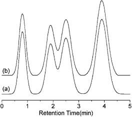
For example, curve (a) in Figure 2.13 is a simulated chromatogram comprising four Gaussian peaks with 512 data points. Curve (b) is reconstructed from the compression data as generated from 10 groups of the parameter set (ai , bi , ci ) for a second-order B-spline function. The relative root mean square error per point as estimated by the following equation is

Figure 2.13. A simulated chromatogram (a) and its profile reconstructed from the compressed data (b).

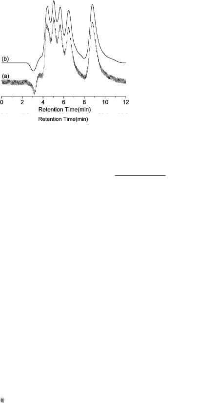
Figure 2.14. An experimental chromatogram (a) and the reconstructed profile using 40 elementary functions (b).

only 0.0012:

Curves (a) in Figures 2.14 and 2.15 are two experimental chromatograms with 900 and 2384 data points, respectively, while curves (b) are profiles

Figure 2.15. An experimental chromatogram (a) and the reconstructed profile using 20 elementary functions (b).

64 one-dimensional signal processing techniques in chemistry

reconstructed by 40 and 20 second-order B-spline functions. The compression ratio is as high as 7.5 : 1 and 39.7 : 1, respectively. From Figure 2.15, it can also be seen that the noise was filtered out during reconstruction. Therefore, such an approach can be used to smooth and compress analytical signals at the same time.

2.4.2.Data Compression Based on Fourier Transformation

As mentioned in Section 2.2, the major feature of Fourier transformation is its transformation of the analytical signals from the time or space domain into the frequency domain. Thus it can also be used for data compression. The principle of compressing the analytical signal by FT is quite simple. It is mainly because the spectra or analytical signals are generally of lower frequency in nature. Consequently, if one keeps only the low-frequency part after transforming the signal into the frequency domain, the signals can be compressed. An example is given here for illustration.

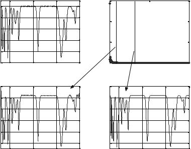
Figure 2.16 gives illustrates how the Fourier transformation is used to compress an infrared spectrum. Curve (a) gives the original simulated infrared spectrum with 3401 data points, while curve (b) shows the result of Fourier transformation on the spectrum from 1 to 1000 frequency points. If only 80 low-frequency points are retained, the recovery signal thus obtained is given as curve (c). It can be seen that the signal reconstructed by using inverse Fourier transformation is quite similar to the original one with a slight distortion. Curve (d) gives the recovery signal with a cutoff threshold frequency of 300 low-frequency points with more data retained compared to the former one following Fourier transformation. It should be noted that the recovery spectrum (Fig. 2.16d) is almost the same as the original one. In this way, an infrared spectrum with 3401 data points can be represented by a data vector containing only 300 low-frequency points with minimal loss of information of the original spectrum. Thus, we can just store these 300 points instead of all the 3401 data of the original spectrum to save the memory space in computer. The procedure of data compression by Fourier transformation is quite similar to that of smoothing the analytical signal. Hence, no source MATLAB code for data compression is provided here.

2.4.3. Data Compression Based on Principal-Component Analysis

In general, principal-component analysis (PCA) is utilized in chemometrics to solve mainly the problem of calibration and resolution. PCA is used to

Figure 2.16. Illustration of how the Fourier transformation can be applied to compress a simulated infrared spectrum. The original simulated IR spectrum (a), the dependence of intensity on frequency after Fourier transformation (b), the recovery signal with the cutoff threshold frequency of 80 low-frequency points (c), and the recovery signal with the cutoff threshold frequency of 300 frequency points (d).

decompose the matrix of interest into several independent and orthogonal principal components. The mathematical formula of principal-component analysis can be expressed as follows.

where U Vt is the singular value decomposition of the matrix X (see Chapter 5 for more detail). The ui and vi values (i = 1, 2, . . . , A) are the so-called score and loading vectors, respectively, and are orthogonal with each other. The diagonal matrix collects the singular values, which are equal to the square root of the variance (eigenvalues of the covariance matrix Xt X, i.e., λi terms arranged in decreasing order) distributing on every orthogonal principal component axis.

It should be noted that the score and loading vectors are orthogonal to each other and their importance is decided by their corresponding eigenvalues (variance). If datasets of spectra or chromatograms in the matrix

66 one-dimensional signal processing techniques in chemistry

retention time points

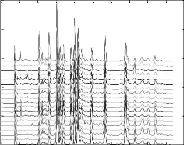
Figure 2.17. Chromatographic fingerprints of 19 Ginkgo biloba samples.

form can be represented by a few loading (or score) vectors, data compression by PCA is possible. A simple example is given here to illustrate the data compression procedure of PCA.

Figure 2.17 shows 19 chromatographic fingerprints of Ginkgo biloba from different pharmaceutical companies obtained by using highperformance liquid chromatography (HPLC). To store these fingerprints, it seems that all of them have to be included. Could we use PCA to help us to save the memory space of our computer? The answer is ‘‘Yes.’’ Let us see how this can be achieved.

The procedure of PCA data compression can be carried out through the following steps:

1.Decompose the data matrix (or dataset) of the analytical signal by PCA to the singular value decomposition [Eq. (2.74)].

2.Find the number of principal components to be retained for reconstructing the original signal later.

3.Store the desirable number of loadings of the largest eigenvalue and the corresponding scores.

Figure 2.18. Illustration of how PCA can be applied for data compression. From top to bottom:

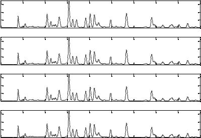
(a) the reconstructed profile of one chromatographic fingerprint by PCA with the first two loadings; (b) the reconstructed profile of one chromatographic fingerprint by PCA with the first three loadings; (c) the reconstructed profile of one chromatographic fingerprint by PCA with the first four loadings; (d) the reconstructed profile of one chromatographic fingerprint by PCA with the first five loadings. Solid blue line---the original fingerprint; dotted red line---the reconstruction fingerprint by PCA.

From this procedure, it can be easily seen that only a few principal loadings and scores are needed to be archived after the PCA treatment. For instance, the variance of the first four principal loadings accounts for 98.32% of the total variance of the 19 samples. Thus, the data to be stored will be the first four principal loadings and the corresponding scores. In comparison to the original dataset, the space for storing the principal loadings and scores for reconstruction is significantly reduced.

Figure 2.18 illustrates the quality of the chromatographic profiles obtained by reconstructing the original analytical signals by different amount of data derived from the principal-component analysis. From these plots, one can see that the chromatographic profile reconstructed by four principal components is good enough because the recovery fingerprint (dotted line) is almost the same as the original one (solid line).

It is worth noting that a new mathematical technique called wavelet transform (WT) has been proposed for signal processing in various fields of analytical chemistry owing to its efficiency and speed in data treatment since 1989 [23--25]. Data compression with the use of WT will be discussed in detail in Chapter 5 in this book.

68 one-dimensional signal processing techniques in chemistry

REFERENCES

1.A. Savitsky and M. J. E. Golay, Anal. Chem. 36:1627 (1964).

2.J. Steinier, Y. Termonia, and J. Deltour, Anal. Chem. 44:1906 (1972).

3.P. A. Gorry, Anal. Chem. 62:570 (1990).

4.S. Rutan, Chemometr. Intell. Lab. Syst. 6:191 (1989).

5.S. D. Brown, Anal. Chim. Acta 181:1 (1986).

6.D. L. Massart, B. G. M. Vandeginste, S. N. Deming et al., Chemometrics: A Textbook, Elsevier, Amsterdam, 1989.

7.A. G. Marshall and M. B. Comisarow, ‘‘Multichannel methods in spectroscopy,’’ in Transform Techniques in Chemistry, P. R. Griffiths, ed., Plenum Press, New York, 1978, Chapter 3.

8.J. Zupan, S. Bohance, M. Razinger et al., Anal. Chim. Acta 210:63 (1988).

9.R. W. Ramirez, The FFT Fundamentals and Concepts, Prentice-Hall, Englewood Cliffs, NJ, 1985.

10.J. W. Cooper, ‘‘Data handling in Fourier transform spectroscopy,’’ in Transform Techniques in Chemistry, P. R. Griffiths, ed., Plenum Press, New York, 1978, Chapter 4.

11.E. O. Brigham, The Fast Fourier Transform, Prentice-Hall, Englewood Cliffs, NJ, 1974.

12.P. R. Griffiths and J. A. De Haseth, Fourier Transform Infrared Spectroscopy, Wiley, New York, 1986.

13.B. K. Alsberg and O. M. Kvalheim, ‘‘Compression of Nth-order data arrays by B-splines. 1. Theory,’’ J. Chemometr. 7(1):61--73 (1993).

14.B. K. Alsberg, E. Nodland, and O. M. Kvalheim, ‘‘Compression of Nthorder data arrays by B-splines. 2. Application to 2nd-order Ft-Ir spectra,’’ J. Chemometr. 8(2):127--145 (1994).

15.X. G. Shao, F. Yu, H. B. Kou, W. S. Cai, and Z. X. Pan, ‘‘A wavelet-based genetic algorithm for compression and de-noising of chromatograms,’’ Anal. Lett. 32(9):1899--1915 (1999).

16.E. F. Crawford and R. D. Larsen, Anal. Chem. 49:508--510 (1977).

17.R. B. Lam, S. J. Foulk, and T. L. Isenhour, Anal. Chem. 53:1679--1684 (1981).

18.P. M. Owens and T. L. Isenhour, Anal. Chem. 55:1548--1553 (1983).

19.F. T. Chau and K. Y. Tam, Comput. Chem. 18:13--20 (1994).

20.C. P. Wang and T. L. Isenhour, Appl. Spectrosc. 41:185--194 (1987).

21.E. R. Malinowski, ed., Factor Analysis in Chemistry, 2nd ed., Wiley, New York, 1991.

22.G. Hangac, R. C. Wieboldt, R. B. Lam, and T. L. Isenhour, Appl. Spectrosc. 36:40--47 (1982).

23.X. D. Dai, B. Joseph, and R. L. Motard, in Wavelet Application in Chemical Engineering, R. L. Motard and B. Joseph, eds., Kluwer Academic Publishers, 1994, pp. 1--32.

24.F. T. Chau, T. M. Shih, J. B. Gao, and C. K. Chan, Appl. Spectrosc. 50:339--349 (1996).

25.K. M. Leung, F. T. Chau, and J. B. Gao, Chemometr. Intell. Lab. Syst. 43: 165--184 (1998).