

Chau Chemometrics From Basics to Wavelet Transform
.pdfintroduction to wavelet transform and wavelet packet transform 109
with the following properties2
|
|
|
∞ |
|
|
|
|
|
lim |
|
|
Sj |
2 |
(4.12) |
|||
|
|
= L (R) |
||||||
j →−∞ Sj = j |
|
|||||||
|
|
|
=−∞ |
|
|
|
|
|
|
∞ |
|
|
|
|
|
|
|
j |
Sj = {0} |
(4.13) |
||||||
|
=−∞ |
|
|
|
|
|
|
|
f (x ) S0 f |
x |
|
Sj |
(4.14) |
||||
|
|
|||||||
2j |
|
|||||||
and there exists a function φ(x ) belonging to L2(R) whose integer translates
{φ(x − k ) | k = . . . , −2, −1, 0, 1, 2, . . . } |
(4.15) |
is an orthonormal basis3 in L2(R). We also say that φ(x ) generates a multiresolution signal decomposition {Sj }.
The term fj (x ) is the representation of f on the scale space Sj and contains all details of f (x ) up to finer resolution level j . For example, if the most accurate ruler used is a millimeter ruler, then we obtain a length approximation only down to a millimeter. Property (4.12) says that the signal approximation fj (x ) from Sj converges to an original signal f (x ) when j → −∞ (the precision becomes finer and finer). You can imagine that fj is the most accurate length to the length f (x ) in all measurable lengths Sj under possible rulers; on the other hand, when j → +∞ (the precision becomes coarser and coarser), Equation (4.13) implies that we lose all the details in the signal f (x ). We cannot measure a length with bigger and bigger rulers. Property (4.14) means that Sj is the 2j scale version of S0 by changing scale and Sj is spanned by the scaled functions
φ |
|
(x ) |
|
1 |
φ |
|
x − 2j k |
|
k |
= |
. . . , |
− |
2, |
− |
1, 0, 1, 2, . . . |
|
j ,k |
= √ |
|
2j |
|||||||||||||
|
|
2j |
|
|
|
|
|
|||||||||
|
|
|
|
|
|
|
|
|
|
|
|
|
|
|
|
|
|
|
|
|
|
|
|
|
|
|
|
|
|
|
|
|
|
that is, each element f (x ) in Sj ( j fixed) can be written in the following form:
+∞
f (x ) = cj ,k φj ,k (x )
k =−∞
For the example of measuring a length, property (4.14) means that a length on a larger scale such as meters can be represented by a length on smaller scales such as millimeters.
2A B and A ∩ B are, respectively, the union and intersection of sets A and B; for instance,
let A |
= { |
1, 2, 3 |
} |
and B |
= { |
2, 3, 5, 6 |
} |
, then A |
|
B |
= { |
1, 2, 3, 5, 6 |
} |
and A |
∩ |
B |
= { |
2, 3 |
} |
. |
|
j =−∞ |
S |
j |
||||
|
|
|
|
|
|
|
|
|
|
|
|
|
|
∞ |
|
|||||||||||||
is the union of all the collections S |
|
and |
|
|
S |
|
the intersection of all the |
collections S . |
|
|||||||||||||||||||
j |
j∞=−∞ |
j |
|
|
|
|
|
j |
|
|
||||||||||||||||||
3 |
More generally {φ(x |
|
|
|
|
|
|
|
|
|
|
|
|
|
|
|
|
|
||||||||||
|
− k ) | k = . . . , −2, −1, 0, 1, 2, . . . } may be a Riesz basis. |
|
|
|
|
|
|
|||||||||||||||||||||

110 |
fundamentals of wavelet transform |
The function generating an MRSD is called a scaling function. As any scaling function φ(x ) S0 S−1, φ(x ) can satisfy a scaling equation, that is, there exists a sequence H = {hk | k = . . . , −2, −1, 0, 1, 2, . . . } of real numbers with, just like the relation of a length on different scales, we obtain
√ |
|
|
+∞ |
|
||
|
|
|
|
hk φ(2x − k ) |
|
|
φ(x ) = 2 |
|
|
(4.16) |
|||
|
|
|
k =−∞ |
|
||
where the coefficients hk can be calculated as |
|
|||||
|
|
|
√ |
|
|
|
hk = φ(x ), 2φ(2x − k ) |
(4.17) |
|||||
This scaling equation relates a scaling function φ(x ) to integer translates of its half-scale versions φ−2,k (x ). The sequence H = {hk | k = . . . , −2, −1, 0, 1, 2, . . . } in scaling equation might be interpreted as a discrete filter as done in signal processing, called a scaling filter.
Example 4.4. Let φ(x ) be the basic unit step function defined by Equation (4.6). It has been shown that the basic unit step yields a multiresolution signal decomposition. From Equation (4.7) the scaling equation [Eq. (4.16)] can be satisfied by taking
|
1 |
|
if k = 0, 1 |
||
hk = |
|
√ |
|
|
|
|
2 |
|
|||
0 |
|
|
otherwise |
||
Our aim is to construct a wavelet to describe detailed information in a signal, not just to build a multiresolution signal decomposition. The aim of introducing MRSD is to construct a wavelet function, specifically, the rulers for measuring a length. Hence we are really interested in the approximation error between the approximations of f (x ) at the scales j and j − 1, which are respectively equal to their orthogonal projections on Sj and Sj −1. As Sj is included in Sj −1, there is an orthogonal complement of Sj in Sj −1:
Sj −1 = Sj Wj |
(4.18) |
which means that any function in Sj −1 can be split into two orthogonal parts, one in Sj and the other in Wj . How can we understand this methodology? Consider the problem of measuring length again. Suppose Sj −1 is all the length information with the accuracy down to the millimeter scale and Sj is the length information on the meter scale. Then we can see that the information in Sj −1 can be split into the information within Sj and the information exactly on the millimeter scale. Thus our desired ruler on the millimeter scale must lie within the error information between Sj −1 and Sj .
introduction to wavelet transform and wavelet packet transform 111
The subspaces Wj are called wavelet subspaces. Similar to the Haar wavelet, we hope that a wavelet basis can be found in these wavelet subspaces. In fact, Mallat [14], Meyer [16], and others proved that for every MRSD there exists a wavelet function ψ(x ) whose scaled and translated
versions of |
|
= √2j |
|
|
|
|
= |
|
− |
|
− |
|
|||
|
j ,k |
(x ) |
2j |
k |
. . . , |
2, |
|||||||||
ψ |
|
1 |
ψ |
x − 2j k |
|
|
|
|
1, 0, 1, 2, . . . |
||||||
|
|
|
|
|
|
|
|
|
|
|
|
|
|
|
|
|
|
|
|
|
|
|
|
|
|
|
|
|
|
|
|
generate an orthonormal basis of the wavelet subspace Wj for each fixed j Z. This is similar to our rulers for measuring a length. Furthermore, the wavelet function can be explicitly constructed from the scaling function φ(x ). The main conclusion can be expressed as follows.
Main Conclusion. Let φ(x ) be an orthogonal scaling function, satisfying the scaling equation (4.16) with a scaling filter H = {hk |k = . . . ,
−2, −1, 0, 1, 2, . . . }, and generate an MRSD {Sj }−j =+∞∞ . Then the function ψ(x ) S−1, defined by
ψ(x ) = √ |
|
|
+∞ |
+∞ |
|
|
k |
gk φ(2x − k ) = k |
gk φ−1,k (x ), |
(4.19) |
|
2 |
|||||
|
|
|
=−∞ |
=−∞ |
|
with gk |
= ( − 1)1−k h1−k , |
|
|
|
|
|
|||||||
has the following properties: |
|
|
|
|
|
|
|||||||
1. For any fixed j |
|
|
|
|
|
|
|
= |
|
||||
|
ψ |
j ,k |
(x ) |
= √2j |
2j |
k |
. . . |
||||||
|
|
|
1 |
ψ |
x − |
2j k |
|
|
|||||
|
|
|
|
|
|
|
|
|
|
|
|
|
|
|
|
|
|
|
|
|
|
|
|
|
|
|
|
(4.20)
, −2, −1, 0, 1, 2, . . .
is an orthonormal basis for Wj
2. All scaled and translated versions {ψj ,k (x ) | j , k = . . . , −2, −1, 0, 1, 2, . . . } provides an orthonormal basis for L2(R); that is, for any f (x ) L2(R), one has
f (x ) = j |
+∞ |
+∞ |
|
j |
dj ,k ψj ,k (x ) |
(4.21) |
|
|
=−∞ =−∞ |
|
|
where dj ,k = f (x ), ψj ,k (x ) are called the wavelet coefficients.
In the previous equations we called H = {hk | k = . . . , −2, −1, 0, 1, 2, . . . } the scaling filter and G = {gk | k = . . . , −2, −1, 0, 1, 2, . . . } the wavelet filter.
112 |
fundamentals of wavelet transform |
We can use two main strategies to construct a wavelet function ψ(x ).
Strategy 1
1.Give or choose an MRSD {Sj }−j =+∞∞ associated with a scaling function φ(x ) (sometimes defining an MRSD is much easier than directly
constructing a wavelet function).
2. |
Find the coefficients hk of scaling filter H = {hk |k = . . . , −2, −1, |
|
0, 1, 2, . . . } by Equation (4.17). |
3. |
Construct a wavelet function ψ(x ) using Equations (4.19) and (4.20). |
Strategy 2
1.Give a scaling filter H = {hk |k = . . . , −2, −1, 0, 1, 2, . . . } with some necessary properties and generate a scaling function φ(x ) using Equation (4.16).
2.Construct a wavelet function ψ(x ) using Equations (4.19) and (4.20).
4.1.3.Basic Properties of Wavelet Function
The MRSD provides us the techniques for constructing wavelet functions. However, a further question is what kind of wavelet functions are preferred. Most applications of wavelets exploit their ability to efficiently approximate or represent particular classes of signals with few nonzero wavelet coefficients. This applies not only for data compression but also for noise removal in chemical data analysis and fast calculations. The design of wavelet function ψ(x ) must therefore be optimized to produce a maximum number of wavelet coefficients dj ,k = f (x ), ψj ,k (x ) in (4.21) that are close to zero. A signal f (x ) has few nonnegligible wavelet coefficients if most of the fine-scale wavelet coefficients are small. This depends mostly on the smoothness of signal f (x ) and the properties of wavelet function ψ(x ) itself. The following features are very important to a wavelet function with the mentioned optimal property:
Vanishing Moments
A wavelet function ψ(x ) has p vanishing moments if
+∞
x k ψ(x )dx = 0 for 0 ≤ k < p
−∞
Why do we introduce the concept of vanishing moments? Simply speaking, if a wavelet function ψ(x ) has larger vanishing moments, then the wavelet coefficients |dj ,k | of a smooth function f (x ) are much smaller on a larger scale j (or at finer resolution).
wavelet function examples |
113 |
Compact Support
The compact support of a wavelet function ψ(x ) is the maximal interval outside of which wavelet function has zero value. For example, the support of Haar wavelet function ψ(x ) is [0, 1) [see Eq. (4.1)]. In general, the smaller the size of such compact, the fewer the highamplitude wavelet coefficients there are. There exists a relationship between the sizes of support of wavelet function and the corresponding scaling filter. If a scaling filter {hk | k = . . . , −2, −1, 0, 1, 2, . . . } has only nonzero values for N1 ≤ k ≤ N2, then the corresponding wavelet function ψ(x ) has a support of size N2 − N1.
Regularity/Smoothness
The regularity of ψ(x ) is a more complicated mathematical concept. It is related to the definition of Holder¨ continuity and other factors. In this chapter we discuss only continuity and smoothness. For example, the Haar wavelet is an example of discontinous wavelets.
4.2.WAVELET FUNCTION EXAMPLES
In the last section we provided MRSD as a tool to construct some desired wavelet functions. Can any wavelet function be found from a MRSD? The simplest Haar provides us an example that can be constructed by the MRSD generated from a special scaling function: the basic unit step function φ(x ) = 1[0,1)(x ). In this section we are about to build more examples and to provide readers with several wavelet functions for their possible applications.
4.2.1. Meyer Wavelet
As mentioned in the rest of Section 4.1.2, one can construct a wavelet function in the Fourier transform. The Meyer wavelet function ψ(x ) is the first example of a wavelet function given its Fourier transform, found by French mathematician Y. Meyer in the 1980s. The Meyer wavelet function is a frequency band-limited function whose Fourier transform has a compact support, namely, nonzero only in a finite interval of frequency variable ω. It is constructed by using the second strategy. The resultant scaling function φ(x ) is defined by its Fourier transform. In Meyer’s method, only the
Fourier transform |
ˆ ( |
ω |
) of the Meyer wavelet function |
ψ |
(x ) is given. As |
|
ψ |
|
|
the expression is very complicated, we omit it here. Readers can consult Daubechies’s book [10] for further details.
114 |
fundamentals of wavelet transform |
|
|
φ(x) |
ψ(x) |
1 |
|
1 |
|
|
|
|
|
0.5 |
0.5 |
|
|
|
|
0 |
0 |
|
-0.5 |
|
|
|
-0.5 |
0 |
-1 |
-5 |
5 |
-5 |
0 |
5 |
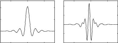
Figure 4.4. Meyer scaling function φ and wavelet ψ.
However, we have no explicit formulas for both the Meyer wavelet function ψ(x ) and the Meyer scaling function φ(x ), although the Fourier transforms of these two functions have been given. Figure 4.4 displays the corresponding Meyer scaling function φ(x ) and Meyer wavelet function ψ(x ). You are encouraged to plot these figures by yourselves with the aid of the MATLAB wavelet toolbox.
Neither the Meyer wavelet function ψ(x ) nor the Meyer scaling function φ(x ) has compact support, that is, ψ(x ) = 0 and φ(x ) = 0 for any x except for some points, but these functions do decrease to 0 when x → ∞ at a very fast speed. Visually they appear as a small wave (see Fig. 4.4), so they can be considered as local waves.
These two functions have better regularity, that is, they are infinitely differentiable, and ψ(x ) has an infinite number of vanishing moments; thus, for any integer m ≥ 0, one has
+∞
x m ψ(x )dx = 0
−∞
4.2.2. B-Spline (Battle--Lemarie) Wavelets
The first strategy is used to construct B-spline wavelet series, assuming a scaling function first. Let Bm (x ) be the box spline of degree m, as in Chapter 2. Bm (x ) can be computed by convolving the basic unit step function 1[0,1) [see Eq. (4.6)] with itself (m + 1) times. It has a compact support centered at 0 or 12 , and is a piecewise polynomial function with (m − 1) times continuous differentiability. Its Fourier transform is
|
|
sin |
ω |
|
m+1 |
Bm (ω) |
|
2 |
e−i (νω/2) |
||
ω |
|
||||
|
= |
2 |
|
|
|
where ν is an indicator whose value is 1 if m is even and 0 if m is odd.

wavelet function examples |
115 |
Let S0 be the set or collection of all the functions consisting of a linear combination of integer translates of Bm (x ); thus, for any f (x ) in S0 one has
f (x ) = ck Bm (x − k )
k Z
Since the integer translates Bm (x − k )s of B-splines are not orthogonal to each other, we need a procedure for constructing a scaling function φ(x ) in S0 whose integer translates are orthogonal to each other so that we can generate an MRSD. The procedure can be arrived at in the Fourier domain. After complicated computation, the procedure gives us a scaling function φm (x ), which can be represented in terms of its Fourier transform. Similarly, the Fourier transform of a B-spline wavelet ψm (x ) can be obtained. Neither of these functions is discussed here; instead, properties of both the scaling filter and the wavelet filter are given. Table 4.1 lists hk corresponding to linear splines m = 1 and cubic splines m = 3 in which the absolute coefficients less than 10−3 are omitted.
The B-spline wavelet function ψm (x ) has (m + 1) vanishing moments and an exponential decay. Since it is generated by a B-spline of degree m, it is (m −1) times continuously differentiable. Although the B-spline wavelet has less regularity than the Meyer wavelet, it has faster asymptotic decay; in other words, the B-spline wavelet is more likely to be a local wave than a Meyer wavelet. Figure 4.5 displays the graph of the cubic spline scaling function φ3(x ) and wavelet ψ3(x ), which is more popular than other B-spline wavelets in actual applications.
Table 4.1. Scaling Coefficients Corresponding to Linear Spline Wavelet and Cubic Spline Wavelet
|
k |
hk |
|
k |
kk |
m = 1 |
0 |
0.817645956 |
m = 3 |
4, −4 |
0.032080869 |
|
1, −1 |
0.397296430 |
|
5, −5 |
0.042068328 |
|
2, −2 |
−0.069101020 |
|
6, −6 |
−0.017176331 |
|
3, −3 |
−0.051945337 |
|
7, −7 |
−0.017982291 |
|
4, −4 |
0.016974805 |
|
8, −8 |
0.008685294 |
|
5, −5 |
0.009990599 |
|
9, −9 |
0.008201477 |
|
6, −6 |
−0.003883261 |
|
10, −10 |
−0.004353840 |
m = 3 |
7, −7 |
−0.002201945 |
|
11, −11 |
−0.003882426 |
0 |
0.766130398 |
|
12, −12 |
0.002186714 |
|
|
1, −1 |
0.433923147 |
|
13, −13 |
0.001882120 |
|
2, −2 |
−0.050201753 |
|
14, −14 |
−0.001103748 |
|
3, −3 |
−0.110036987 |
|
|
|

116 |
fundamentals of wavelet transform |
1.2 |
|
|
|
|
1.5 |
|
|
|
|
|
|
|
|
|
|
|
|
|
|
||
1 |
|
|
|
|
1 |
|
|
|
|
|
0.8 |
|
|
|
|
|
|
|
|
|
|
0.6 |
|
|
|
|
0.5 |
|
|
|
|
|
|
|
|
|
|
|
|
|
|
||
0.4 |
|
|
|
|
0 |
|
|
|
|
|
|
|
|
|
|
|
|
|
|
||
0.2 |
|
|
|
|
|
|
|
|
|
|
0 |
|
|
|
|
-0.5 |
|
|
|
|
|
-0.2 |
|
|
|
|
-1 |
|
|
|
|
|
-10 |
-5 |
0 |
5 |
10 |
-5 |
0 |
5 |
10 |
||
-10 |
Figure 4.5. Cubic spline scaling function φ and wavelet ψ.
4.2.3. Daubechies Wavelets
Daubechies wavelets (see Daubechies wavelets and scaling functions in Fig. 4.6) are commonly used in wavelet analysis. They were developed by mathematician I. Daubechies in 1989. Although Meyer wavelet and spline wavelets are orthogonal, they are not compactly supported; that is, ψ(x ) = 0 for any x except for some points. The Daubechies wavelet is the first example of wavelets with the compactly supported properties. The construction strategy for Daubechies wavelets is to begin with finiteimpulse response filters H = {h0, h1, . . . , hN−1}, which implies that the
φ(x)
1.5 |
|
|
|
1 |
|
|
|
0.5 |
|
|
|
0 |
|
|
|
-0.5 |
|
|
|
0 |
1 |
2 |
3 |
ψ(x)
2 |
|
|
|
1 |
|
|
|
0 |
|
|
|
-1 |
|
|
|
-2 |
1 |
2 |
3 |
0 |
φ(x) |
φ(x) |
1.5 |
|
|
|
|
|
1.5 |
|
|
|
1 |
|
|
|
|
|
1 |
|
|
|
0.5 |
|
|
|
|
|
0.5 |
|
|
|
0 |
|
|
|
|
|
0 |
|
|
|
-0.5 |
1 |
2 |
3 |
4 |
5 |
-0.5 |
2 |
4 |
6 |
0 |
0 |
||||||||
|
|
|
ψ(x) |
|
|
|
|
ψ(x) |
|
2 |
|
|
|
|
|
1.5 |
|
|
|
1.5 |
|
|
|
|
|
1 |
|
|
|
1 |
|
|
|
|
|
|
|
|
|
|
|
|
|
|
0.5 |
|
|
|
|
0.5 |
|
|
|
|
|
|
|
|
|
|
|
|
|
|
|
|
|
|
|
0 |
|
|
|
|
|
0 |
|
|
|
|
|
|
|
|
|
|
|
|
|
-0.5 |
|
|
|
|
|
-0.5 |
|
|
|
-1 |
|
|
|
|
|
|
|
|
|
|
|
|
|
|
|
|
|
|
|
-1.5 |
1 |
2 |
3 |
4 |
5 |
-1 |
2 |
4 |
6 |
0 |
0 |
Figure 4.6. Daubechies scaling functions φ and wavelets ψ.
wavelet function examples |
117 |
transfer function of H is a trigonometric polynomial:
N−1
H(ω) = hk e−ik ω
k =0
Daubechies provided a constructive proof of the existence for such a wavelet function. Take N = 2p, where p is a given order of vanishing moments; then there exists at least a wavelet ψ(x ) with p vanishing moments and support [−p + 1, p], and the corresponding scaling function φ(x ) has the support defined by [0, 2p − 1]. When p = 1, one obtains the Haar wavelet. Daubechies gave a computing method for the filter coefficients hk . Table 4.2 lists all the filter coefficients for p ≤ 7.
We still have no explicit formulas for the scaling function φ(x ) and the wavelet function ψ(x ). The regularity of φ(x ) and ψ(x ) is the same since by the scaling Equation (4.19), ψ(x ) is a finite linear combination of φ−1,k (x ). However, this regularity is difficult to estimate precisely. In general, the Daubechies wavelet is uniformly smooth. For p = 2, the wavelet ψ(x ) is only continuous but nondifferentiable (with Lipschitz order 0.55); for p = 3, the wavelet ψ(x ) is already continuously differentiable.
Daubechies wavelets are very asymmetric. To obtain a symmetric or antisymmetric wavelet, the scaling filter H must be symmetric or antisymmetric with respect to the center of its support. Daubechies has proved that the Haar wavelet is the only one compactly supported classical wavelet whose filter is symmetric or antisymmetric. Daubechies made modifications to her wavelets such that the symmetry of new wavelets can be improved while retaining great simplicity. The resulting wavelets still have a minimum support [−p + 1, p] with p vanishing moments, but they are more symmetric. Those wavelets, called Symmlets, have many properties similar to those of Daubechies wavelets.
4.2.4.Coiflet Functions
Daubechies wavelets are asymmetric. In actual applications, symmetric templates are sometimes preferred. However, Daubechies proved that no wavelet function could exist with the properties of compact support, continuity, and symmetry occurring simultaneously.
Coiflets are wavelet functions with much more symmetry than Daubechies wavelets. A coiflet function ψ(x ) has 2p vanishing moments, and the corresponding scaling function φ(x ) has (2p − 1) vanishing moments. Both functions have a compact support of length (6p − 1).
The coefficients of scaling filters are listed in Table 4.3.
118 |
|
|
fundamentals of wavelet transform |
|||
|
|
Table 4.2. Daubechies Wavelet Coefficients |
||||
|
|
|
|
|
|
|
|
|
k |
hk |
|
k |
kk |
|
|
|
|
|
|
|
|
p = 1 |
0 |
0.707106781 |
p = 6 |
0 |
0.111540743 |
|
p = 2 |
1 |
0.707106781 |
|
1 |
0.494623890 |
|
0 |
0.482962913 |
|
2 |
0.751133908 |
|
|
|
1 |
0.836516304 |
|
3 |
0.315250352 |
|
|
2 |
0.224143868 |
|
4 |
−0.226264693 |
|
p = 3 |
3 |
−0.129409523 |
|
5 |
−0.129766868 |
|
0 |
0.332670553 |
|
6 |
0.097501606 |
|
|
|
1 |
0.806891509 |
|
7 |
0.027522866 |
|
|
2 |
0.459877502 |
|
8 |
−0.031582039 |
|
|
3 |
−0.135011020 |
|
9 |
0.000553842 |
|
|
4 |
−0.085441274 |
|
10 |
0.004777258 |
|
p = 4 |
5 |
0.035226292 |
p = 7 |
11 |
−0.001077301 |
|
0 |
0.230377813 |
0 |
0.077852054 |
||
|
|
1 |
0.714846571 |
|
1 |
0.396539319 |
|
|
2 |
0.630880768 |
|
2 |
0.729132091 |
|
|
3 |
−0.027983769 |
|
3 |
0.469782287 |
|
|
4 |
−0.187034812 |
|
4 |
−0.143906004 |
|
|
5 |
0.030841382 |
|
5 |
−0.224036185 |
|
|
6 |
0.032883012 |
|
6 |
0.071309219 |
|
p = 5 |
7 |
−0.010597402 |
|
7 |
0.080612609 |
|
0 |
0.160102398 |
|
8 |
−0.038029937 |
|
|
|
1 |
0.603829270 |
|
9 |
−0.016574542 |
|
|
2 |
0.724308528 |
|
10 |
0.012550999 |
|
|
3 |
0.138428146 |
|
11 |
0.000429578 |
|
|
4 |
−0.242294887 |
|
12 |
−0.001801641 |
|
|
5 |
−0.032244870 |
|
13 |
0.000353714 |
|
|
6 |
0.077571494 |
|
|
|
|
|
7 |
−0.006241490 |
|
|
|
|
|
8 |
−0.012580752 |
|
|
|
|
|
9 |
0.003335725 |
|
|
|
|
|
|
|
|
|
|
For more details, see Daubechies’s book [10]. We suggest that you explore coiflets using the MATLAB wavelet toolbox.
4.3.FAST WAVELET ALGORITHM AND PACKET ALGORITHM
In this section we introduce the basic algorithm, derived by Mallat [14] for fast computation of the discrete wavelet transform. In practice, any signals from an equipment, such as chemical spectrum, are discrete. Thus the most useful transform should be in discrete version. The discrete wavelet algorithms can be easily derived from the scaling equations. The wavelet