

Brereton Chemometrics
.pdf342 |
CHEMOMETRICS |
|
|
Baseline Peaks
Figure 6.2
Dividing data into regions prior to baseline correction
6.2.2 Principal Component Based Plots
Scores and loadings plots have been introduced in Chapter 4 (Section 4.3.5). In this chapter we will explore some further properties, especially useful where one or both of the variables are related in sequence. Table 6.1 represents a two-way dataset, corresponding to HPLC–DAD, each elution time being represented by a row and each measurement (such as successive wavelengths) by a column, giving a 25 × 12 data matrix, which will be called dataset A. The data represent two partially overlapping chromatographic peaks. The profile (sum of intensity over the spectrum at each elution time) is presented in Figure 6.3.
|
14 |
|
|
|
|
|
|
|
12 |
|
|
|
|
|
|
|
10 |
|
|
|
|
|
|
|
8 |
|
|
|
|
|
|
Intensity |
6 |
|
|
|
|
|
|
|
|
|
|
|
|
|
|
|
4 |
|
|
|
|
|
|
|
2 |
|
|
|
|
|
|
|
0 |
|
|
|
|
|
|
|
1 |
5 |
9 |
13 |
17 |
21 |
25 |
|
−2 |
|
|
Datapoint |
|
|
|
Figure 6.3
Profile of data in Table 6.1
EVOLUTIONARY SIGNALS |
|
|
|
|
|
|
|
|
|
|
|
|
|
|
|
|
|
|
|
|
|
|
|
|
|
343 |
||
|
|
|
|
|
|
|
|
|
|
|
|
|
|
|
|
|
|
|
|
|
|
|
|
|
|
|
|
|
|
L |
|
.0558 |
.0608 |
.048 |
.1521 |
.2164 |
.2212 |
.5579 |
.8741 |
.9038 |
.8434 |
.6739 |
.5869 |
.4386 |
.3938 |
.3639 |
.2178 |
.1021 |
.0979 |
.0307 |
.0308 |
.0017 |
.0653 |
.0072 |
.0853 |
.027 |
|
|
|
|
||||||||||||||||||||||||||
|
|
|
0 0 0 0 0 0 0 0 0 0 0 0 0 0 0 0 0 0 0 0 0 0 0 0 0 |
|
||||||||||||||||||||||||
|
|
|
− |
|
|
|
|
|
|
|
|
|
|
|
|
|
|
|
|
|
|
|
|
− − |
|
|
|
|
|
K |
|
0.0174 |
0.0355 |
0.0283 |
0.1371 |
0.2227 |
0.4225 |
0.5986 |
0.9435 |
0.9545 |
0.9744 |
0.8432 |
0.6549 |
0.4393 |
0.4327 |
0.3217 |
0.2212 |
0.0379 |
0.0518 |
0.0458 |
0.014 |
0.0065 |
0.0026 |
0.0579 |
0.0619 |
0.0237 |
|
|
|
|
|
|
|
|
|
|
|
|
|
|
|
|
|
|
|
|
|
|
|
− |
− |
− |
|
|
|
|
|
J |
|
0.0645 −0.0015 −0.0246 |
0.1275 |
0.1143 |
0.4269 |
0.5496 |
0.8334 |
0.8645 |
0.9224 |
0.7912 |
0.6313 |
0.5641 |
0.6646 |
0.4457 |
0.3343 |
0.1546 |
0.0491 |
0.0129 −0.0342 |
−0.0138 |
−0.0186 |
0.0242 −0.0236 |
0.003 |
|
||||
|
I |
|
−0.032 −0.0034 |
0.0293 |
0.0669 |
0.1024 |
0.341 |
0.529 |
0.5212 |
0.7138 |
0.7661 |
0.78 |
0.7796 |
0.959 |
0.9459 |
0.7724 |
0.5951 |
0.3231 |
0.1289 |
0.1577 |
0.0152 |
−0.0222 |
0.0038 |
0.0072 −0.0368 |
0.0156 |
|
||
|
H |
|
0.0459 |
0.1377 |
0.0259 |
0.0587 |
0.1367 |
0.1325 |
0.3343 |
0.334 |
0.5695 |
0.5333 |
0.7855 |
1.0237 |
1.2283 |
1.2238 |
1.1237 |
0.7876 |
0.5677 |
0.2925 |
0.1047 |
0.1182 |
0.0975 |
0.0383 |
0.0342 |
0.0182 |
0.0263 |
|
|
|
|
− |
|
− − |
|
|
|
|
|
|
|
|
|
|
|
|
|
|
|
|
|
− |
|
|
− |
|
|
|
G |
|
0.0518 |
0.0123 |
−0.0612 |
0.0499 −0.0015 |
0.1919 |
0.3703 |
0.3584 |
0.5764 |
0.7043 |
0.907 |
1.1164 |
1.3362 |
1.3713 |
1.3094 |
0.9616 |
0.582 |
0.3571 |
0.1721 |
0.0213 |
0.0218 |
0.0479 |
0.0263 −0.0018 −0.0137 |
|
|||
|
F |
|
.0336 |
.0377 |
.0528 |
.1912 |
.1575 |
.293 |
.3783 |
.6825 |
.7215 |
.793 |
.9552 |
.1321 |
.2339 |
.3175 |
.1592 |
.8509 |
.4634 |
.2974 |
.2454 |
.0468 |
.0053 |
.0716 |
.0507 |
.0946 |
.0236 |
|
|
|
|
0 0 0 0 0 0 0 0 0 0 0 1 1 1 1 0 0 0 0 0 0 0 0 0 0 |
|
||||||||||||||||||||||||
|
|
|
− − |
|
|
|
|
|
|
|
|
|
|
|
|
|
|
|
|
|
|
− |
|
− |
|
|
|
|
|
E |
|
.0079 |
.072 |
.0386 |
.0185 |
.2383 |
.3234 |
.6054 |
.0843 |
.1767 |
.1986 |
.0619 |
.094 |
.9656 |
.9758 |
.7807 |
.5427 |
.2747 |
.1922 |
.0113 |
.0693 |
.0648 |
.067 |
.0199 |
.0572 |
.0291 |
|
|
|
|
0 0 0 0 0 0 0 1 1 1 1 1 0 0 0 0 0 0 0 0 0 0 0 0 0 |
|
||||||||||||||||||||||||
|
|
|
− |
|
|
|
|
|
|
|
|
|
|
|
|
|
|
|
|
|
− |
|
− |
|
|
|
− |
|
|
D |
|
.0622 |
.0014 |
.0009 |
.1073 |
.3531 |
.7042 |
.0167 |
.3823 |
.5951 |
.5679 |
.254 |
.0496 |
.7349 |
.5837 |
.4609 |
.3332 |
.1721 |
.1622 |
.0239 |
.0564 |
.0405 |
.0533 |
.0052 |
.0046 |
.0395 |
|
|
|
|
0 0 0 0 0 0 1 1 1 1 1 1 0 0 0 0 0 0 0 0 0 0 0 0 0 |
|
||||||||||||||||||||||||
|
|
|
|
− − |
|
|
|
|
|
|
|
|
|
|
|
|
|
|
|
− − − − |
|
|
|
|
||||
|
C |
|
.0886 |
.0507 |
.1005 |
.1828 |
.4304 |
.7367 |
.3239 |
.6344 |
.9253 |
.5299 |
.2793 |
.8139 |
.5844 |
.3344 |
.169 |
.1684 |
.079 |
.0842 |
.0672 |
.0362 |
.0371 |
.0323 |
.0175 |
.0191 |
.0185 |
|
|
|
|
0 0 0 0 0 0 1 1 1 1 1 0 0 0 0 0 0 0 0 0 0 0 0 0 0 |
|
||||||||||||||||||||||||
|
|
|
− |
|
|
|
|
|
|
|
|
|
|
|
|
|
|
|
|
|
− − |
|
|
|
− |
|
|
|
6.1 DatasetA. |
A B |
|
0.1102 −0.0694 −0.0487 0.0001 |
0.036 0.0277 |
0.2104 0.1564 |
0.1713 0.3206 |
0.497 0.6192 |
0.6753 1.1198 |
1.0412 1.5129 |
1.0946 1.5543 |
0.9955 1.4794 |
0.672 1.1315 |
0.469 0.7531 |
0.3113 0.3894 |
0.0891 0.2121 |
0.0567 0.1408 0.0391 −0.0211 0.0895 −0.0086 0.007 −0.024 0.0146 −0.0567 0.0012 −0.0043 −0.0937 0.0324 −0.0031 0.0127 |
−0.0387 −0.0041 −0.0449 0.0076 −0.0986 0.0244 |
|
||||||||||
Table |
|
|
1 |
2 |
3 |
4 |
5 |
6 |
7 |
8 |
9 |
10 |
11 |
12 |
13 |
14 |
15 |
16 |
17 |
18 |
19 |
20 |
21 |
22 |
23 |
24 |
25 |
|
|
|
|
|
|
|
|
|
|
|
|
|
|
|
|
|
|
|
|
|
|
|
|
|
|
|
|
||
344 |
|
|
|
|
|
|
|
|
|
|
CHEMOMETRICS |
|
|
2 |
|
|
|
|
|
|
|
|
|
|
|
1.5 |
|
|
|
|
15 |
14 |
|
|
|
|
|
|
|
|
|
|
13 |
|
|
|
|
|
PC2 |
|
|
|
|
16 |
|
|
|
|
|
|
1 |
|
|
|
|
|
|
|
|
||
|
|
|
|
|
|
|
|
|
|
||
|
|
0.5 |
|
|
17 |
|
|
|
12 |
|
|
|
|
19 |
|
18 |
|
|
|
|
|
|
|
|
|
|
|
|
|
|
|
|
|
||
|
|
0 |
|
|
|
|
|
|
|
11 3.5 |
|
−0.5 |
|
0 |
4 0.5 |
1 |
1.5 |
2 |
2.5 |
3 |
4 |
||
|
|
−0.5 |
|
|
5 |
|
PC1 |
|
|
|
|
|
|
|
|
|
6 |
|
|
|
|
|
|
|
|
|
|
|
|
|
|
|
|
10 |
|
|
|
|
|
|
|
|
|
7 |
|
|
|
|
|
−1 |
|
|
|
|
|
|
|
9 |
|
|
|
|
|
|
|
|
|
|
|
||
|
|
|
|
|
|
|
|
|
|
|
|
|
|
|
|
|
|
|
|
|
|
8 |
|
|
|
−1.5 |
|
|
|
|
|
|
|
|
|
|
|
0.6 |
|
|
|
|
|
|
|
|
|
|
|
|
|
|
|
|
|
H |
|
G |
|
|
|
0.4 |
|
|
|
|
|
|
|
|
|
|
|
|
|
|
|
|
|
|
F |
|
|
|
|
|
|
|
|
|
|
|
|
|
|
|
|
0.2 |
|
|
|
|
|
I |
|
|
|
|
|
|
|
|
|
|
|
|
|
|
|
PC2 |
|
|
|
|
|
|
|
|
|
E |
|
|
0 |
|
|
|
|
|
J |
|
|
|
|
|
|
|
|
|
|
|
|
|
|
|
|
|
|
|
0 |
|
|
PC1 |
0.2 |
|
|
|
0.4 |
|
|
|
|
|
|
|
L |
K |
|
|
D |
|
−0.2 |
|
|
|
|
|
|
|
|
||
|
|
|
|
|
|
|
A |
|
|
|
|
|
−0.4 |
|
|
|
|
|
|
|
B |
C |
|
|
|
|
|
|
|
|
|
|
|
|
|
|
−0.6 |
|
|
|
|
|
|
|
|
|
|
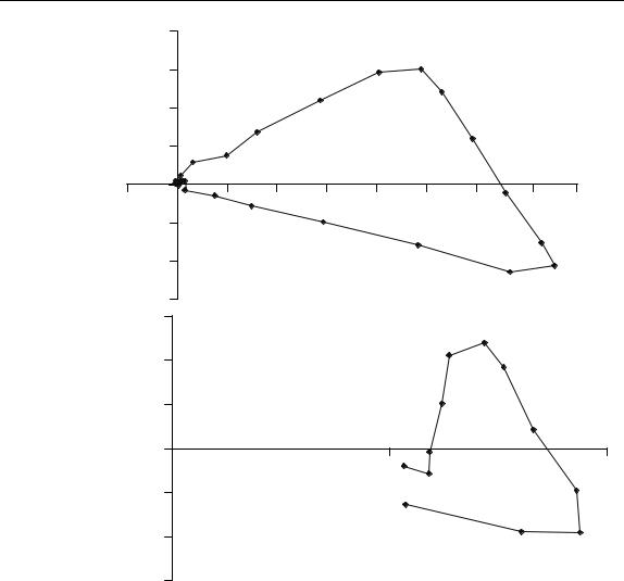
Figure 6.4
Scores and loadings plots of PC2 versus PC1 of the raw data in Table 6.1
The simplest plots are the scores and loadings plots of the first two PCs of the raw data (see Figure 6.4). These would suggest that there are two components, with a region of overlap between times 9 and 14, with wavelengths H and G most strongly associated with the slowest eluting compound and wavelengths A, B, C, L and K with the fastest eluting compound. For further discussion of the interpretation of these types of graph, see Section 4.3.5.
The dataset in Table 6.2 is of the same size but represents three partially overlapping peaks. The profile (Figure 6.5) appears to be slightly more complex than that for dataset A, and the PC scores plot presented in Figure 6.6 definitely appears to contain more features. Each turning point represents a pure compound, so it appears that there are three compounds, centred at times 9, 13 and 17. In addition, the spectral characteristics
EVOLUTIONARY SIGNALS |
|
|
|
|
|
|
|
|
|
|
|
|
|
|
|
|
|
|
|
|
|
|
|
|
|
345 |
||
|
|
|
|
|
|
|
|
|
|
|
|
|
|
|
|
|
|
|
|
|
|
|
|
|
||||
|
L |
|
0.0784 −0.0746 −0.0437 |
0.0614 |
0.1335 |
0.2801 |
0.7223 |
0.8289 |
0.8584 |
0.8324 |
0.8146 |
0.5917 |
0.6865 |
0.9762 |
1.2778 |
1.7106 |
1.8048 |
1.6280 |
1.1998 |
0.6602 |
0.1539 |
0.0798 |
0.0518 −0.0489 −0.0383 |
|
||||
|
|
|
||||||||||||||||||||||||||
|
K |
|
0.0641 −0.0715 −0.0654 |
0.1128 |
0.1688 |
0.3498 |
0.6187 |
0.8351 |
1.0880 |
0.9573 |
0.7305 |
0.6364 |
0.7354 |
0.8967 |
1.2267 |
1.5703 |
1.6209 |
1.4607 |
1.0083 |
0.4253 |
0.2760 |
0.0782 |
−0.0521 |
0.0664 |
0.0480 |
|
||
|
J |
|
−0.0257 −0.0295 −0.0271 |
0.0396 |
0.0472 |
0.3195 |
0.4346 |
0.8600 |
1.0155 |
1.0264 |
0.9810 |
0.7335 |
0.7738 |
0.8656 |
0.9667 |
1.1937 |
1.1376 |
0.9945 |
0.6982 |
0.2982 |
0.2204 |
0.0370 |
0.0217 |
−0.1066 |
0.0319 |
|
||
|
I |
|
0.0078 −0.0341 −0.0079 |
0.0421 |
0.0898 |
0.1049 |
0.3163 |
0.6141 |
0.7866 |
0.7726 |
0.9984 |
0.9874 |
0.9871 |
0.9289 |
0.9415 |
0.8331 |
0.6828 |
0.5582 |
0.3016 |
0.2330 |
0.1284 |
0.0411 |
−0.0036 |
−0.0119 |
−0.0279 |
|
||
|
H |
|
0.0066 |
0.0876 |
0.1114 |
0.0499 |
0.0657 |
0.0382 |
0.1802 |
0.3650 |
0.4519 |
0.6486 |
0.9789 |
1.1761 |
1.3346 |
1.2373 |
0.8403 |
0.6494 |
0.3421 |
0.2421 |
0.1631 |
0.0176 |
0.0322 |
0.0517 |
0.0282 |
0.0258 |
0.0358 |
|
|
|
|
− |
|
− − |
|
|
|
|
|
|
|
|
|
|
|
|
|
|
|
|
|
− |
− − |
|
|
||
|
G |
|
0.0530 |
0.0074 |
0.0365 |
0.0396 |
0.0310 |
0.1147 |
0.1340 |
0.2991 |
0.4163 |
0.6598 |
0.9594 |
1.3408 |
1.3799 |
1.2870 |
0.9244 |
0.5775 |
0.2725 |
0.1154 |
0.0062 |
0.0121 |
0.0367 |
0.1068 |
0.0374 |
0.0199 |
0.1094 |
|
|
|
|
− |
|
|
|
|
|
|
|
|
|
|
|
|
|
|
|
|
|
|
− |
|
|
|
|
− |
|
|
F |
|
0.0404 |
0.0218 |
0.0102 −0.0213 |
0.0886 |
0.0725 |
0.2480 |
0.3124 |
0.3880 |
0.6088 |
0.9031 |
1.2316 |
1.2065 |
1.1305 |
0.7994 |
0.4061 |
0.1431 |
0.0917 |
0.0012 −0.0078 |
0.0410 |
0.0023 |
−0.1177 −0.0066 |
0.0637 |
|
|||
|
E |
|
0.0399 |
−0.1072 |
−0.0347 |
0.0045 |
0.1594 |
0.1596 |
0.3413 |
0.5933 |
0.6591 |
0.7743 |
0.8587 |
0.9716 |
1.0398 |
0.8882 |
0.5563 |
0.2568 |
0.1279 |
0.1297 |
−0.0290 −0.0180 |
0.0239 |
0.0017 |
0.0020 −0.0212 |
−0.0511 |
|
||
|
D |
|
0.0136 |
−0.0251 |
−0.0229 |
−0.0142 |
0.1567 |
0.3477 |
0.6515 |
0.9179 |
1.1441 |
1.1872 |
0.9695 |
0.8352 |
0.6098 |
0.5386 |
0.3367 |
0.2574 |
0.1255 |
0.0936 |
0.0071 |
0.0714 |
−0.0689 |
−0.0307 |
−0.0867 −0.0875 |
0.0298 |
|
|
|
C |
|
−0.0059 |
0.0183 |
−0.0246 |
−0.0155 |
0.1601 |
0.5696 |
0.9926 |
1.3641 |
1.5372 |
1.5099 |
1.0579 |
0.7074 |
0.5143 |
0.3630 |
0.2429 |
0.3146 |
0.3203 |
0.1603 |
0.1668 |
0.0825 |
0.0436 |
0.0418 |
0.0520 −0.0536 |
0.0093 |
|
|
6.2 DatasetB. |
A B |
|
−0.1214 0.0097 |
0.0750 −0.0200 |
−0.0256 0.1103 |
0.0838 0.0486 |
0.1956 0.2059 |
0.4605 0.5753 |
0.9441 1.1101 |
1.3161 1.6053 |
1.5698 1.8485 |
1.3576 1.6975 |
1.0215 1.1341 |
0.5267 0.6154 |
0.3936 0.3650 |
0.4351 0.3077 |
0.7120 0.4754 |
1.0076 0.5493 |
1.2155 0.5669 |
1.1392 0.4750 |
0.6988 0.4000 |
0.3291 0.1766 |
0.2183 0.1892 |
0.1135 0.0517 |
−0.0442 0.0156 |
−0.0013 −0.1103 |
0.0697 0.0827 |
|
Table |
|
|
1 |
2 |
3 |
4 |
5 |
6 |
7 |
8 |
9 |
10 |
11 |
12 |
13 |
14 |
15 |
16 |
17 |
18 |
19 |
20 |
21 |
22 |
23 |
24 |
25 |
|
|
|
|
|
|
|
|
|
|
|
|
|
|
|
|
|
|
|
|
|
|
|
|
|
|
|
|
||


EVOLUTIONARY SIGNALS |
347 |
|
|
|
|
2 |
|
|
|
|
|
|
|
|
|
|
|
1.5 |
|
|
|
|
|
|
13 |
|
|
|
|
|
|
|
|
|
|
12 |
|
|
|
|
|
|
|
|
|
|
|
|
|
|
|
|
PC2 |
1 |
|
|
|
|
|
|
14 |
|
|
|
|
|
|
|
|
|
|
|
|
||
|
|
|
|
|
|
|
|
|
|
|
|
|
|
|
|
|
|
|
|
|
11 |
|
|
|
|
0.5 |
|
|
|
|
|
|
|
|
|
|
|
|
|
|
|
PC1 |
|
|
15 |
10 |
|
|
|
0 |
|
|
|
|
|
|
|
||
|
|
|
|
|
|
|
|
|
|
|
|
−0.5 |
|
0 |
0.5 |
1 |
1.5 |
2 |
2.5 |
3 |
3.5 |
4 |
|
|
−0.5 |
|
21 |
6 |
|
7 |
|
8 |
9 |
|
|
|
|
|
|
|
|
|
|
||||
|
|
|
|
|
20 |
|
|
|
16 |
|
|
|
|
−1 |
|
|
|
19 |
|
|
|
|
|
|
|
|
|
|
|
|
|
17 |
|
|
|
|
|
|
|
|
|
|
|
18 |
|
|
|
|
−1.5 |
|
|
|
|
|
|
|
|
||
|
|
|
|
|
|
|
|
|
|
||
|
0.6 |
|
|
|
|
|
|
|
|
|
|
|
0.4 |
|
|
|
|
|
F |
G |
|
|
|
|
|
|
|
|
|
H |
|
|
|
||
|
|
|
|
|
|
|
E |
|
|
|
|
|
0.2 |
|
|
|
|
|
|
D |
|
|
|
|
|
|
|
|
|
|
|
I |
|
|
|
|
|
|
|
|
|
|
|
|
|
|
|
PC2 |
0 |
|
|
|
|
PC1 |
|
|
C |
|
|
|
|
|
|
|
|
|
|
|
|||
|
|
|
|
|
|
|
|
|
|
||
|
0 |
|
|
|
|
0.2 |
|
|
|
0.4 |
|
|
|
|
|
|
|
|
|
B |
|||
|
−0.2 |
|
|
|
|
|
|
|
J |
|
|
|
|
|
|
|
|
|
|
|
|
|
|
|
|
|
|
|
|
|
|
|
|
A |
K |
|
−0.4 |
|
|
|
|
|
|
|
|
L |
|
|
|
|
|
|
|
|
|
|
|
||
|
−0.6 |
|
|
|
|
|
|
|
|
|
|
Figure 6.6
Scores and loadings plots of PC2 versus PC1 of the raw data in Table 6.1
about terminology. If only two PCs are used this will project the scores on to a circle, whereas if three PCs are used the projection will be on to a sphere. It is best to set A according to the number of compounds in the region of the chromatogram being studied.
Figure 6.9 illustrates the scores of dataset A normalised over two PCs. Between times 3 and 21, the points in the chromatogram are in sequence on the arc of a circle. The extremes (3 and 21) could represent the purest elution times, but points influenced primarily by noise might lie anywhere on the circle. Hence time 25, which is clearly


 −2
−2


 −0.4
−0.4
350 |
|
|
|
|
|
|
CHEMOMETRICS |
|
|
|
1.2 |
|
|
|
|
|
|
21 |
1 |
20 |
|
|
|
|
|
19 |
|
|
|
||
|
|
|
|
|
|
|
|
|
|
|
0.8 |
22 |
|
|
|
|
|
|
|
|
|
|
|
|
|
|
|
|
17 |
|
|
|
|
|
0.6 |
|
16 |
|
|
|
|
|
|
18 |
15 |
|
|
|
|
|
|
|
14 |
|
|
|
|
1 |
|
|
|
24 |
|
|
|
0.4 |
|
|
2 |
|
|
|
|
|
|
|
13 |
|
|
|
|
|
|
|
|
23 |
|
|
|
|
0.2 |
|
|
12 |
|
|
|
PC2 |
|
|
|
|
|
|
|
|
0 |
|
|
11 |
|
−1.5 |
−1 |
−0.5 |
|
|
|
|
|
0 |
0.5 |
|
1 |
1.5 |
|||
|
|
|
−0.2 |
PC1 |
|
10 |
|
|
|
|
|
|
|
9 |
|
|
|
|
−0.4 |
|
|
678 |
|
|
|
|
|
|
5 |
|
|
|
|
|
|
|
|
4 |
|
|
|
|
−0.6 |
|
|
|
|
|
|
|
−0.8 |
25 |
3 |
|
|
|
|
|
−1 |
|
|
|
|
Figure 6.9
Scores of dataset A normalised over the first two principal components
•the purest points for the middle eluting peak are 12 and 13, again a turning point;
•the purest points for the slowest eluting peak are 18–20;
•points 23–25 are mainly dominated by noise.
It is probably best to remove the noise points 1–4 and 23–15, and show the normalised scores plot as in Figure 6.10(b). Notice that we come to a slightly different conclusion from Figure 6.6 as to which are the most representative elution times (or spectra) for each component. This is mainly because the ends of each limb in the raw scores plot correspond to the peak maxima, which are not necessarily the purest regions. For the fastest and slowest eluting components the purest regions will be at more extreme elution times before noise dominates: if the noise levels are low they may be at the base rather than top of the peak clusters. For the central peak the purest region is still at the same position, probably because this peak does not have a selective or pure region. The data could also be normalised over three dimensions with pure points falling on the surface of a sphere; the clustering becomes more obvious (see Figure 6.11). Note that similar calculations can be performed on the loadings plots and it is possible to normalise the loadings instead.
6.2.3 Scaling the Data
It is also possible to scale the raw data prior to performing PCA.
6.2.3.1 Scaling the Rows
Each successive row in a data matrix formed from a coupled chromatogram corresponds to a spectrum taken at a given elution time. One of the simplest methods of scaling
