Cohen M.F., Wallace J.R. - Radiosity and realistic image synthesis (1995)(en)

CHAPTER 9. RENDERING

9.5 MAPPING RADIOSITIES TO PIXEL COLORS

Figure 9.21: The goal is to match the perception.

minance is, transformed to perceived brightness, Bdisp, through the process of perception by the observer. This is represented by the display observer, which transforms luminance to brightness under the conditions of viewing a CRT.

The goal is to derive a tone reproduction operator that makes Bdisp, as close to Brw as possible. Such an operator can be constructed using the concatenation of three operators:

1.the real-world observer, (i.e., the perceptual transformation from simulated luminance, Lrw, to brightness, Brw),

2.the inverse of the display observer, (i.e., the transformation of Bdisp to Ldisp ), and

3.the inverse of the display device operator, (i.e., the transformation from display luminance, Ldisp, to the required pixel value, V).

CHAPTER 9. RENDERING

9.5 MAPPING RADIOSITIES TO PIXEL COLORS

Applying these three operators in sequence transforms the simulated luminance to a pixel value that can be sent to the frame buffer. The inverse operators in this sequence effectively undo the subsequent application of the display and observer operators in advance, thus making the net overall transformation from simulated luminance to perceived brightness equivalent to applying only the real world observer. Since the real world observer transforms Lrw to Brw, the result is the desired match.

Tumblin and Rushmeier formulate the above real-world and display observer operators using an observer model based on the work of Stevens [225]. Stevens’ model expresses the relationship between luminance, Lin, and perceived brightness B by

where α and β account for the observer’s adaptation to the overall image luminance, Lw. This equation provides the model for both the real-world observer and the display observer, with different α and β in each case corresponding to the adaptation levels for the different viewing conditions. The α and β parameters are given by

α(Lw) = 0.41 log10(Lw) + 2.92

(9.16)

β(Lw) = –0.41(log10 (Lw ))2 + (–2.584 log10Lw) + 2.0208

where Lw approximates the average overall luminance of the viewed real world scene in one case and of the synthesized image in the other.

The display operator is expressed in terms of the contrast between a displayed luminance Ldisp and the maximum displayable luminance Ldmax:

where V is the pixel value in the frame buffer, and Cmax is the maximum contrast between onscreen luminances. The γ in Vγ is the gamma term for

video display described earlier. The 1/Cmax term accounts for the effect of ambient light falling on the screen on image contrast. The Cmax term is defined by the ratio of brightest to dimmest pixels, typically a value of about 35 : 1.

Combining equations 9.15 and 9.17 and inverting them where called for, a single operator is derived that takes a luminance, Lrw , to a pixel value, V:

This relation maps the results of the global illumination simulation into a “best” choice of pixel values, thus providing the last step in the image synthesis process.

CHAPTER 9. RENDERING

9.5 MAPPING RADIOSITIES TO PIXEL COLORS

Figure 9.22. Images produced after accounting for brightnesses and viewer adaptation based on work by Tumblin and Rushmeier. Light source intensities range from 10–5 lamberts to 103 lamberts in geometrically increasing steps by 100. Coutesy of Jack Tumblin, Georgia Institute of Technology.

The advantage of using equation 9.18 is demonstrated in Figure 9.22 for a model in which the light source ranges in intensity from 10–5 lamberts to 103 lamberts in geometrically increasing steps. Linear scaling would generate the lower left image no matter what the light source energy. Using Tumblin and Rushmeier’s tone reproduction operator, the sequence successfully (and automatically) reproduces the subjective impression of increasingly bright illumination.

If hardware rendering is used to create the image, it will obviously be impossible to perform a sophisticated mapping to the radiosity at every pixel. Instead, the nodal radiosities will have to be transformed before they are sent to the hardware as polygon vertex colors. The result will differ somewhat from the foregoing, since the pixel values in this case will be obtained by linear interpolation from the mapped values, while the mapping itself is nonlinear.

As Tumblin and Rushmeier point out, the observer model upon which this operator is based simplifies what is in reality a very complex and not completely understood phenomenon. For example, color adaptation is ignored. There is also the question of what adaptation luminance to use in computing the α and β terms. Tumblin and Rushmeier use a single average value over the view or screen, but further research might explore whether or not the adaptation level

CHAPTER 9. RENDERING

9.6 COLOR

should be considered constant over the field of view.

However, this work is an important step toward quantifying the perceptual stage of the image synthesis process. The significance of such quantitative models lies in their ultimate incorporation into the error metrics that guide the solution refinement. Current metrics, for example, may force mesh refinement in regions that are bright and washed out in the image, and thus contain little visible detail. The goal of a perceptually based error metric would be to focus computational effort on aspects of the solution only to the extent that they affect image quality.

9.6 Color

The topic of color has been ignored in the previous chapters partly because it is a complex topic in its own right, and partially because it is not integral to the explanation of the radiosity method. Each of the issues addressed in the earlier chapters is valid (with a few provisos7), for a full color world as well as a monochrome one. The geometric quantities such as the form factor are independent of material properties like color. The solution process is independent of color in as much as a separate solution can be performed for each wavelength or color band of interest.

A full description of color and color perception cannot be provided here. Instead, interested readers are referred to a number of excellent sources for more detail [156]. Valuable information from researchers in image synthesis can be found in [114, 166].

Questions of immediate interest addressed in this section are,

•What and how many wavelengths or color bands should be used in the radiosity solution?

•Can a single scalar value be used for error criteria, and if so, how is a reasonable achromatic value derived from the color model?

•How can one transform values between color models to finally derive RGB pixel values?

The following sections outline properties of human color perception and how these relate to the selection of color models. A color model provides a framework to specify the color of light sources and reflective surfaces. Color

70ne assumption in this process is that light of one wavelength is not reflected at another. With the exception of fluorescent materials, this assumption is not violated. It has also been assumed that light that is absorbed is not reemitted in the visible spectrum. This again is true at “normal” temperatures.

CHAPTER 9. RENDERING

9.6 COLOR

models are used at three stages in the radiosity simulation: (l) as part of the description of the environment to be rendered, (2) during the radiosity solution, and (3) during the creation of the final image on the output device. The same or different color models may be used at each of these stages. Different color models and means to transform values between them are discussed below.

The selection of a color model for the radiosity solution depends on the required accuracy of the color reproduction and available information about the lights and surfaces contained in the input to the simulation. For example, if colors are input in terms of red, green, and blue components, then the simulation can proceed by computing red, green, and blue radiosity values at each node. The results can then be mapped directly to the RGB phosphors on a CRT based on the specific properties of the monitor. However, this simple RGB color model contains inherent limitations that make it difficult or impossible to reproduce exactly the subtleties of color in the real-world. A fuller description of the visible energy (light) at each point requires a specification of the energy at all wavelengths in the visible spectrum. If a full (or sampled) spectrum of the emitted energy of light sources and of the reflectivity of materials is available, methodologies can be developed that lead to more accurate color simulations.

9.6.1 Human Vision and Color

The normal human eye is sensitive to electromagnetic radiation (light) at wavelengths between approximately 380 and 770 nanometers. The familiar rainbow presents the spread of the visible spectrum from the short (blue) to the long (red) wavelengths. Light leaving a surface and entering the eye will generally contain some energy at all wavelengths in the visible spectrum. The relative amounts of energy at each wavelength determine the color we see. For example, equal amounts of energy at all wavelengths produce a sensation of white light.

It might at first seem that producing an accurate color image would require reproducing the complete details of the energy across the visible spectrum, in other words, the amount of energy at each wavelength at each point on the environment’s surfaces.

Fortunately for the image synthesis process the human visual system greatly simplifies the problem. Experiments have shown that very different energy spectra can produce identical color sensations. Two different spectra that produce the same sensation are called metamers. The reasons for this phenomenon and the way in which this fact can be taken advantage of in the image synthesis process are discussed below.

CHAPTER 9. RENDERING

9.6 COLOR

Figure 9.23: Luminous efficiency function.

Luminous Efficiency Function

The eye is not equally sensitive to light of different wavelengths even within the visible portion of the electromagnetic spectrum. The luminous efficiency function (see Figure 9.23) describes the eye’s sensitivity to light of various wavelengths and can be used to convert between radiance, which is independent of perceptual phenomena, and the perceptual quantity, luminance.8

Thus, when working in an achromatic context (black and white), it is best to multiply the energy spectrum by the luminous efficiency function to obtain a scalar luminance value that can be displayed as a gray value or used as a decision variable for element subdivision. As will be discussed below, certain color models contain one channel devoted to carrying achromatic luminance information and are thus a convenient model for image synthesis. Scalar luminance values can also be derived from sampled wavelength-based models by weighting the energy at each sample wavelength by the corresponding value in luminous efficiency function.

Color Sensitivity

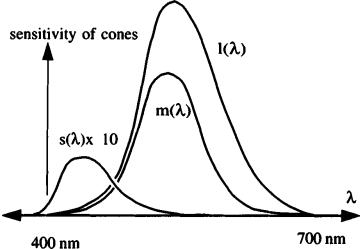
Color perception results from receptors in the eye called cones. It has been found that normal human eyes have only three types of cones, each with distinct responses to light across the visible spectrum (see Figure 9.24). One type of cone is sensitive primarily to short (S) wavelengths, one to medium (M) wavelengths, and the other to longer (L) wavelengths. Color blindness is believed to be caused

8The corresponding units of measure from the fields of radiometry and photometry are discussed in Chapter 2.

CHAPTER 9. RENDERING

9.6 COLOR

Figure 9.24: Response of three color cones in eye (after Meyer, 1986).

by a deficiency in one or more of the three cone types. It is the response of colorblind individuals to color that has provided much of the evidence of the three distinct color cones.

The fact that color perception appears to be a function of only three stimulus values provides the basis for metamerism. If two light spectra, when integrated against the cone response functions, result in the same three values, then the human eye is unable to distinguish between them. This is the root of metamerism and is of great help in image synthesis since it provides a basis to produce a wide range of color sensations by combining only a very few sources. In particular, combinations of light produced by the red, green, and blue phosphors of the typical CRT can recreate most possible color sensations.

9.6.2 Color Matching Functions and the CIE Chromaticity Diagram

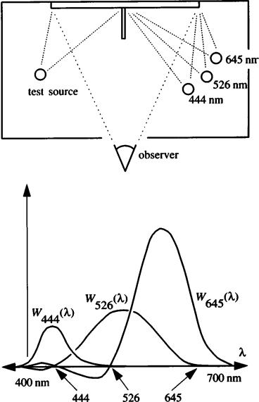
Given the above observation, a three dimensional color space can be organized. Experiments, as depicted in Figure 9.25, have been conducted in which an observer is shown light from a monochromatic (single wavelength) test source, and is simultaneously shown the combined light from three other monochromatic sources or primaries chosen at short, medium, and long (s, m, l) wavelengths. The observer is allowed to adjust the (s, m, l) primaries until there is a match. One can then plot the resulting amounts of the three primaries as the test source wavelength is varied across the visible spectrum resulting in three color matching functions, (s(l), m(l), l(l)). Although most test sources can be matched by a positive combination of the three adjustable sources, some cannot be matched. In this case, the observer is allowed to move one of the three primaries to the left

CHAPTER 9. RENDERING

9.6 COLOR

Figure 9.25: Color matching experiment and resulting color matching functions.

side and add it to the test source. This quantity is then counted as a “negative” amount of that primary.

The three resulting matching functions now provide all the information required to match not only the monochromatic test sources, but any combination of energy across the spectrum. A general spectrum E(l) can be represented with a linear combination of the primaries (s, m, l) given by

CHAPTER 9. RENDERING

9.6 COLOR

Figure 9.26: CIE standard observer matching functions.

where

In fact, the three matching functions can be replaced by any three independent linear combinations of the original three matching functions, resulting in a new color space defined by new matching functions. These can be used in exactly the same way as the results of the original matching experiment.

A commonly used set of matching functions was developed in 1931 by the Commission Internationale de l’Éclairage (CIE) based on the “standard observer’s” matching functions. The CIE functions, x(λ), y(λ), and z(λ), are shown in Figure 9.26. These were chosen such that the XYZ color space contains all possible spectra in the positive octant and y(λ) corresponds to the luminous efficiency function.

Figure 9.27 shows the CIE XYZ color space. A direction emanating from the origin in this space represents all multiples of a particular linear combination of the three matching functions. Within the limits discussed in section 9.5, the points along a line from the origin will all produce the same color sensation at different brightnesses. The horseshoe-shaped curve indicates the directions in the space corresponding to the set of monochromatic sources (i.e., the rainbow)