Cohen M.F., Wallace J.R. - Radiosity and realistic image synthesis (1995)(en)

CHAPTER 9. RENDERING

9.3 TWO-PASS METHODS

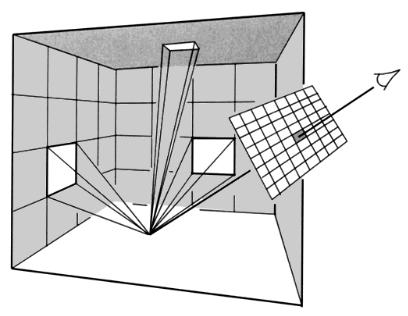
Figure 9.15: Monte Carlo ray tracing, using the radiosity approximation to determine radiance for secondary rays.

More generally, the computation of B(xp ) using equation 9.9 can be restricted to locations in the image where the visible element has been identified during the solution as liable to be inaccurate, according to any of the error metrics discussed in Chapters 6 and 7. In the hierarchical formulation of Chapter 7, one might go a step farther and only reevaluate the integral for specific interactions that involve partial visibility and a large amount of energy.

Evaluating the integral of equation 9.8 at each pixel requires considerable computation since it involves form factor type computations from the point xp . Most of the form factor algorithms discussed in Chapter 4 are applicable. Several algorithms using this approach are described in the following sections.

Monte Carlo Ray Tracing per Pixel

Rushmeier [198] describes a two-pass approach in which the first pass consists of a constant element radiosity solution. During the rendering pass the rendering equation is evaluated using Monte Carlo path tracing [135], with paths limited to one bounce (see Figure 9.15). Multiple rays are traced from the eye through each pixel into the scene. From the intersection point of each ray, a single ray is traced to a random point on a light source and a second ray is traced in a

CHAPTER 9. RENDERING

9.3 TWO-PASS METHODS

Figure 9.16: An image computed using Monte Carlo path tracing, with the radiosity solution supplying the radiance at secondary ray intersections. Courtesy of Holly E. Rushmeier, Program of Computer Graphics, Cornell University.

random direction chosen with a probability proportional to the cosine of the angle measured from the normal.

The radiance at the point intersected by the secondary ray is obtained from the radiosity solution. If the secondary ray hits a light source, it must be counted as making a contribution of zero, since the sources are already accounted for by the ray to the light. The final pixel color resulting from n rays through the pixel is then

where the ith ray from the eye intersects the environment at xi , the secondary ray from xi to a light intersects the source at xiL and the secondary ray reflected randomly from xi intersects the environment at

Rushmeier points out that meshing algorithms can be greatly simplified when the radiosity solution is no longer required to capture shading features like shadows in great detail. As with all Monte Carlo solutions, noisy images will occur if too few sample rays are used. Figure 9.16 shows an image computed using Rushmeier’s algorithm.

CHAPTER 9. RENDERING

9.3 TWO-PASS METHODS

Figure 9.17: Computing form factors to every element at every pixel to compute the final bounce of the radiosity equation.

Form Factors per Pixel

In a two-pass method described by Reichert [192], the radiosity at each pixel is computed by evaluating a form factor to every element in the radiosity mesh (see Figure 9.17). This is ultimately less efficient than Rushmeier’s Monte Carlo approach, since it computes a contribution from every element, regardless of its contribution to the pixel variance. For the same reason, however, this approach has the advantage of never missing an important source of illumination. Although expensive, it produces images of extremely high quality (see Figure 9.18.)

Reichert notes that although meshing requirements for the radiosity solution are less rigorous when the final bounce is evaluated at image resolution, sampling in image space can exacerbate certain types of errors. For example, the illumination provided by constant elements can cause shading artifacts for nearby receivers (see Figure 9.19 (a)). Similarly, coherent errors introduced by the form factor evaluation used at each pixel may create highly visible patterns in the image, as shown in Figure 9.19 (b), where form factors are computed with point sampling. Monte Carlo integration of the form factor may be preferable in this case since it will produce noise that is less objectionable than coherent errors.

CHAPTER 9. RENDERING

9.3 TWO-PASS METHODS

Figure 9.18: Image computed by evaluating form factors at each pixel to every element. Courtesy of Mark Reichert, Program of Computer Graphics, Cornell University.

Figure 9.19: (a) Artifacts caused by pixel-by-pixel form factor evaluation in

proximity to large discontinuities in ˆ . The high gradients on the wall near

B

the floor correspond to the boundaries of constant elements on the floor. (b) Artifacts caused by coherent errors in the form factor evaluation. Courtesy of Mark Reichert, Program of Computer Graphics, Cornell University.

CHAPTER 9. RENDERING

9.3 TWO-PASS METHODS

Figure 9.20: Shooting rays to compute the direct component of illumination during rendering. The direct component is interpolated from the radiosity solution.

Direct Illumination per Pixel

It is not necessary in a two-pass method to integrate over all the elements that provide illumination. Typically only a few such elements contribute to high frequencies in the image. Integration can be limited to these elements, with the contribution of the remainder interpolated from the radiosity solution. Shirley [212] describes a two-pass method based on this approach in which only the contribution of direct illumination (illumination from light emitters) is recomputed by integration during rendering. Direct illumination typically arrives from small relatively high energy sources and is thus more likely to produce high gradients in the radiance function, which generally require fine sampling for accurate approximation. Indirect illumination usually arrives from relatively low energy sources distributed over a large solid angle and is thus less likely to create high gradients.

Shirley computes the indirect component of illumination in a first pass consisting of a modified progressive radiosity solution, during which the direct and indirect components are stored separately. In the second pass the direct component of the radiosity function is reevaluated at each image pixel using Monte Carlo sampling of the light emitters (see Figure 9.20). This is added to the indirect component interpolated from the radiosity mesh. An example, which also incorporates bump mapping and specular reflections, is shown in color plate 41.

CHAPTER 9. RENDERING

9.3 TWO-PASS METHODS

Kok al. [141] describe a generalization of this approach in which illumination due to the most significant secondary reflectors as well as the emitters is recomputed during rendering, based on information gathered during the radiosity pass.

9.3.2 Multi-Pass Methods

Although two-pass methods take advantage of the view to focus computational effort, they have limitations. While two-pass approaches can account for high frequencies across surfaces with respect to the final reflection of light to the eye, they also assume that the global first pass radiosity solution is a sufficiently accurate approximation of the secondary illumination for the particular view. Two-pass methods provide no mechanism for recognizing when this assumption is violated and, when it is, for refining the first-pass solution accordingly. In splitting the solution into separate view-dependent and view-independent passes, two-pass methods explicitly break the connection that would ultimately allow automatic refinement of the solution to achieve an image of a specified accuracy. The importance meshing algorithm of Smits et al. [220] addresses this problem directly.

The multi-pass method described by Chen et al. [52] is a generalization of the two-pass method that offers another approach to overcoming this limitation. In the multi-pass algorithm, the radiosity solution is merely the initial step of a progressive rendering process. Over a sequence of steps the radiosity approximation is eventually replaced by a Monte Carlo solution at each pixel (with specular reflection also accounted for in later passes). The use of multiple steps allows finely tuned heuristics to be used to determine where and when to commit computational resources in creating an increasingly accurate image. However, care must be taken in designing a multi-pass method. In particular:

1.Redundant energy transport must be avoided. Each possible path for light transfer must be accounted for only once. This may require removing part of the radiance computed in an earlier pass before summing in a more accurate estimate. Transport paths are discussed in more detail in the Chapter 10.

2.Heuristics should be unbiased. In the limit, as more computational resources are used, the solution should always converge to the true solution. This is often a subtle and difficult aspect to assess.

Color plates 35-39 show the improvement of images with successive passes of Chen’s algorithm.

CHAPTER 9. RENDERING

9.4 INCORPORATING SURFACE DETAIL

9.4 Incorporating Surface Detail

In the discussion of the radiosity method so far it has been assumed that surface properties such as reflectivity are constant over each surface, or at least over the support of an individual basis function or element. This has allowed the reflectivity term to be moved outside the integral during the computation of the linear integral operator.

Surface detail is often simulated in image synthesis by using a texture map to specify the variation over the surface of properties such as reflectivity, transparency or the surface normal. Techniques for incorporating texture mapping and bump mapping (mapping the surface normal) into radiosity algorithms are described in the next sections.

9.4.1 Texture Mapping

When surface reflectivity is specified by a texture map, the resulting shading typically contains very high spatial frequencies. These are difficult to represent adequately with a finite element approximation. As an alternative, during the radiosity solution the reflectivity r of a texture mapped surface can be approximated by the average texture reflectivity (the texture color), ρ , over the support of a basis function. This is a reasonable assumption in most cases, since high frequency variations in radiance are averaged together during integration.4

During rendering, computing the radiosity at a particular point on a texture mapped surface requires knowing the incident energy (irradiance) at that point. This is computed explicitly in the two-pass methods previously discussed, and texture maps are handled trivially in such methods. However, even if the radiosities are interpolated from the solution, it is still possible to extract an approximation of the incident energy.

For elements on a texture mapped surface, the nodal radiosities will have

The radiosity is simply multiplied by the texture mapped reflectivity for the pixel over the average reflectivity [61]. This effectively undoes the multiplication of

4This assumption can be violated when a texture mapped surface containing large scale variations in color is located near another surface, For example, a floor with a black and white tile pattern may produce noticeable shading variations on the wall near the floor due to light reflected from the tiles.

CHAPTER 9. RENDERING

9.5 MAPPING RADIOSITIES TO PIXEL COLORS

the incident energy by the average reflectivity ρ that was performed during the solution and then multiplies the incident energy by the reflectivity ρ(xp ) specified for that location by the texture map. The paintings in Color Plates 10, 13, 17, and 22 as well as the floor tiles in color plate 45 are texture maps incorporated into the image using this technique.

It is also possible to combine texture mapping with radiosity using hardware accelerators that support texture mapping. This is discussed in section 9.7, where the details of rendering radiosity using hardware graphics accelerators are described.

9.4.2 Bump Mapping

A bump map represents variations in the surface normal using an array of values mapped to the surface, analogously to a texture map. Like texture maps, bump maps generally produce shading with high spatial frequencies. Hence, by nature, bump maps are best handled by per-pixel shaders. Two-pass methods handle bump maps in a straightforward manner by using the perturbed normal at each pixel during the view pass when computing the final radiosity. The image by Shirley (color plate 41), includes a bump mapped brick pattern that was added during the rendering pass [213].

It is also possible to support bump mapping when interpolation is used for rendering. During the solution, instead of computing a single radiosity value at each node, the variation of radiosity with surface orientation at the node is sampled by computing independent radiosity values for several surface normals distributed over the hemisphere. During rendering, the perturbed normal at a particular pixel is determined from the bump map. For each of the element nodes, the radiosity corresponding to that orientation is interpolated from the hemisphere sampling, and the radiosity at the pixel is bilinearly interpolated from these nodal values.

Chen [49] implements this algorithm by applying the hemicube gathering approach. A single hemicube is computed at each node. The form factors for each sampled surface orientation are computed from this hemicube by resumming the delta form factors, which are modified from the usual values to correspond to the new surface orientation. Chen samples 16 surface orientations at each node.

9.5 Mapping Radiosities to Pixel Colors

Having finally computed a radiance at every pixel, the remaining rendering step consists of assigning a corresponding frame buffer pixel value, typically an integer in the range of 0 to 255. If color is desired, the radiosity solution will have been computed at several wavelengths, and the mapping will include

CHAPTER 9. RENDERING

9.5 MAPPING RADIOSITIES TO PIXEL COLORS

a transformation to the red-green-blue (RGB) color space of the monitor. The monochrome issues will be addressed first, followed by a short discussion of color.

The ultimate goal is to construct an image that creates the same sensation in the viewer as would be experienced in viewing the real environment. As discussed in the introductory chapter, there are many obstacles to realizing this ideal, most of which are not unique to image synthesis. These include the nonlinear relationship between voltage and luminance in the display device, the restricted range of luminance values available on the display, limited color gamut, the ambient lighting conditions under which the image is viewed, as well as the basic limitations of representing three-dimensional reality as a projection onto a two-dimensional image plane.5

9.5.1 Gamma Correction

The first difficulty encountered is that monitors, in general, do not provide a linear relationship between the value specified at a frame buffer pixel (which determines the voltage of the electron gun at that pixel) and the resulting screen radiance. Rather, the radiance, I, is related to voltage, V, by [84],

The value of γ varies between monitors, but is usuaully about 2.4 ± 0.2. Thus

Therefore, assuming that the target radiance is in the available dynamic range of the monitor, a voltage must be selected from the available discrete voltages,

The adjustments for the nonlinear relationship between voltage and radiance through the use of the exponent, 1/γ, is called gamma correction.

9.5.2 Real-World Luminance to Pixel Luminance

A more challenging problem is the limited dynamic range of the display device. Luminance values experienced in the real-world range from 10–5cd/meter2 (starlit forest floor) to 10 5 cd/meter2 (sun reflected off snow). In contrast, a typical CRT can display luminances in the range of only 1 to 100 cd/meter. It is therefore necessary to map the values produced by the radiosity simulation to the

5These issues are covered in much greater detail in Hall’s monograph [114].

CHAPTER 9. RENDERING

9.5 MAPPING RADIOSITIES TO PIXEL COLORS

range available on the CRT. The goal is to produce a subjective impression of brightness in viewing the image on a CRT that is equivalent to that experienced in viewing the real environment.

One simple approach is to map the luminance values in the radiosity solution linearly to the luminance range of the monitor. Unfortunately, the only thing visible in images produced using a linear mapping will usually be the light source, since its luminance is typically several orders of magnitude greater than that of any reflecting surface. Radiosity implementations often get around this by mapping the highest reflected luminance (as opposed to the light sources) to slightly less than the maximum pixel value and set the light sources themselves to the maximum value. The “slightly less” ensures that light sources appear brighter than any reflecting surface.

This mapping is completely arbitrary, and it is thus difficult to judge from the image what the appearance of the real environment might be under equivalent lighting conditions. Tumblin and Rushmeier [238] demonstrate this using the example of a room illuminated by a light emitting with the power of a firefly versus a room illuminated by a light with the same geometry, but with the power of a searchlight. Because of the linearity of the integral operator in the rendering or radiosity equations, scaling each resulting luminance range by the maximum reflected luminance will produce identical images!

What is required is a tone reproduction operator, which will transform luminances to frame buffer values in such a way that the perceived brightness of the image equals that experienced by a hypothetical observer viewing a real scene having the same luminances. Tumblin and Rushmeier derive such an operator from simple models of the display and viewing processes. Their work is a good example of how a model of perception might be incorporated into image synthesis.

Figure 9.21 contains a diagram of the processes of perceiving real-world and synthesized scenes. In the real-world, the luminance of the scene, Lrw, is received by the eye and converted to a subjective perceived brightness, Brw.6 This is represented by the real world observer, which transforms luminance to brightness under the conditions of viewing in the real world.

For a simulated scene, the computed luminance (which is assumed to closely approximate the real-world luminance, Lrw), is mapped to a frame buffer pixel value, V, (assumed here to be a number ranging from 0.0 to 1.0) by the tone reproduction operator, which is to be derived. The pixel value is then transformed by the display operator to a displayed luminance, Ldisp. Finally, displayed lu-

6Luminance measures light energy in terms of the sensitivity of a standard human eye, and is computed by integrating the spectral radiance weighted by the luminous efficiency curve for the eye over the visual spectrum (see Chapter 2). Brightness is a measure of the subjective sensation created by light.