

Microcontrollers in Practice (Mitescu M., 2005)
.pdf14
PI Temperature Controller
14.1 In this Chapter
This chapter is an introduction to the basic principles of control systems. It also contains a description of a didactic implementation of a PI temperature controller that uses the HC11 development board described in Chap. 9.
14.2 Basic Concepts
A control system is a system comprising physical and decisional elements, designed to control (to interferewith, to influence, to modify) a process.
In the classic example of a switch that controls an electric heater, the human operator has both decision and execution functions. A system where the intervention of a human operator is required is called manual control. If in this example the human operator is replaced by a time relay that switches the heater on and off at predetermined time intervals, the system becomes an automatic sequential system.
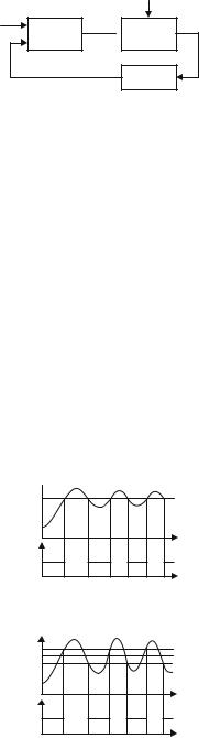
This system does not check whether the controlled heater actually produces heat, and the temperature of the environment does not influence the time relay. When the interaction between the control system and the controlled process is unidirectional, the control system is called an open-loop control system (see Fig. 14.1) .
Open-loop control systems are often associated with manual control. Most automatic control systems have at least one active feedback loop which allows the system to evaluate the response of the controlled process and adjust the control action, so that the value of a controlled variable is maintained close to a set-point value. The general block diagram of a closed-loop control system is shown in Fig. 14.2.
CONTROL Vout  PLANT
PLANT
Fig. 14.1. Block diagram of an open-loop control system
174 14 PI Temperature Controller
Disturbances
Vs
Vm CONTROL Vout  PLANT
PLANT
SENSOR
Fig. 14.2. General structure of a closed-loop control system
In this configuration, the sensor measures the value Vm of the process variable (which can be temperature, pressure, speed, flow, pH, etc.) and submits it to the control unit, which compares it to the desired value, or set-point value Vs, and adjusts the output Vout to reduce the error e = Vs − Vm.
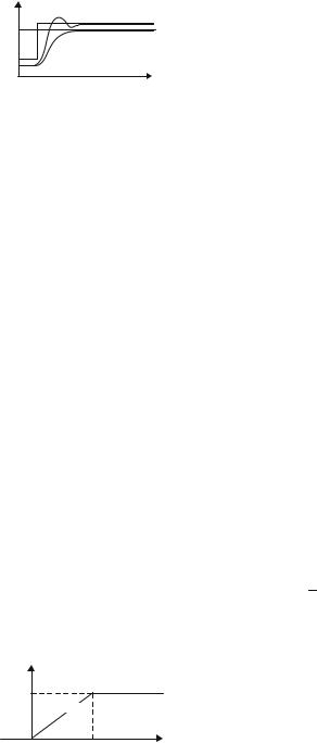
Figure 14.3 describes the simplest control algorithm, where the controlled process variable is the temperature. The output of the control circuit Vout turns the heating element on, when the measured temperature Tm is lower than the set-point temperature Ts, and off, when Tm > Ts.
In practice, the turn-on (T1) and turn-off (T2) threshold temperatures are deliberately made to differ by a small amount (called hysteresis), to prevent switching of the heating element rapidly and unnecessarily, when the measured temperature Tm is close to the set-point value Ts (refer to Fig. 14.4). Most domestic thermostats use this control algorithm.
The problem with the on–off control systems is that the fluctuations of the controlled process variable are often too large to be acceptable. A better solution, from this point of view, is proportional control. In this case, the output of the control circuit Vout adjusts the power applied to the heater in proportion to the error signal
Tm 
Ts
t
Vout
t
Fig. 14.3. Waveforms for the on–off control
Tm
T2
Ts
T1
t
Vout
t
Fig. 14.4. On–Off control with hysteresis
14.2 Basic Concepts |
175 |
Tm
Kp2>Kp1
Ts
Te
Kp1
t
Fig. 14.5. Waveforms for proportional control
e(t) = Ts − Tm: |
|
Vout = Kp × e(t) . |
(14.1) |
Kp is called the proportional gain of the control circuit. The response of this system to a step change of the set-point temperature is shown in Fig. 14.5.
For moderate values of Kp, and in the absence of disturbances, the system reaches a steady state temperature Te < Ts, when the energy brought into the system by the heater compensates the energy losses. The steady state error (Ts − Te) can be reduced by increasing Kp, but higher values for Kp cause overshoot, or oscillations of the controlled temperature around the set-point value. In fact, for very large values of Kp, the proportional control acts like the on–off control described above. The reason for that is that the heating can only supply a limited power Vmax, and it cannot sink power when Tm > Ts.
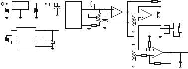
Therefore, when Kp is very large, Vout = Vmax, even for small values of the error e(t), as shown in Fig. 14.6. The interval of values for e(t) where Vout takes values in proportion to e(t) is called the proportional band (PB).
The expression (14.1) reflects only the status of the system at the present time. To solve the problem of the steady state error, it is required to adjust V out by adding a term that reflects the evolution of the error in the past. Mathematically, this is expressed by the integral of the error over a period of time. The output of a proportional-integral (PI) control system is described by:
t |
|
Vout = Kp × e(t) + Ki × e(t)dt |
(14.2) |
0
The constant Ki is called the integral gain. Often, Ki is represented as Ki = 1 ,
Ti
where Ti is called integral time constant of the control system. The response of this system to a step change of the set-point temperature is shown in Fig. 14.7.
Vout |
|
Vmax |
Vout=Vmax |
|
|
Vout=Kp*e(t) |
|
Vout=0 |
|
PB e(t)=Ts-Tm
Fig. 14.6. The output of a proportional control system

176 14 PI Temperature Controller
Tm
Kp2>Kp1
Ts
Kp1
t
Fig. 14.7. Response of a PI control system to a step change in the error
The effect of the integral term is to adjust the output of the control circuit, until the time-averaged error is zero. Note that if the error e(t) is large for a long period, for example after a large change of the set-point, or at start-up, then the value of the integral of the error becomes too large, and causes overshoot that takes a long time to recover. One method to avoid this problem (which is called integral wind-up) is to inhibit integral action while the error is outside the proportional band.
The integral action solves the problem of the steady state error, but not the problem of overshoot. In principle, by keeping Kp at relatively low values it is possible to avoid the overshoot, at the expense of a slow response of the system, as shown in Fig. 14.8, curve 1.
To reduce the response time, it is required to adjust Vout by adding a new term to the expression (14.2). This term should be proportional to the speed of variation of the error, e(t), which is the first derivative of e(t). The expression for Vout becomes:
|
t |
de(t) |
|
||
Vout = Kp × e(t) + Ki × |
e(t)dt + Kd × |
(14.3) |
|||
|
. |
||||
dt |
|||||
|
0 |
|
|
|
|
This is the general expression of the output of a proportional-integral-derivative control system (PID). Kd is called the derivative gain, or damping factor. The derivative term only affects Vout when the error has a fast variation, for example when the set-point value is changed. In steady state, the value of the derivative term is zero. The effect of the derivative term on the response of the system is presented in Fig. 14.8, curve 2.
While the proportional term in the expression for Vout describes the present status of the system, and the integrative term is related to the past evolution of the system, the derivative contains information about the tendency of evolution of the system in the future. Negative values of the derivative mean that the error is decreasing, i.e. the controlled parameter tends to approach the set-point value, and therefore the control
Tm
Ts
21
t
Fig. 14.8. Two possible responses to a step change in the error
14.3 Hardware Implementation of a Microcontroller-Based Temperature Controller |
177 |
action Vout is reduced. This explains the damping effect of the derivative component on the oscillations of the response of the system around the set-point value.
Temperature control systems are in most cases inherently slow-response systems, and therefore the derivative component is seldom useful for temperature control. Moreover, in noisy environments, some noise spikes can be misinterpreted as step changes of the error, and induce instability in the whole system. For these reasons, the example of the temperature controller described in this chapter is a PI type controller.
14.3 Hardware Implementation of a Microcontroller-Based
Temperature Controller
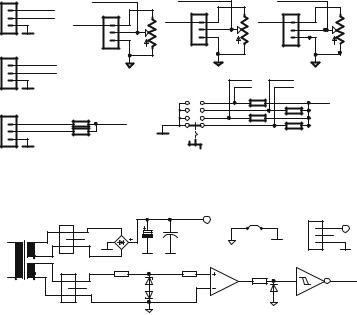
The hardware implementation of the temperature controller uses the HC11 development board described in Chap. 9, along with an expansion board containing the circuits for interfacing the temperature sensor and the heater. The schematic of the interface with the temperature sensor is presented in Fig. 14.9.
The actual temperature sensor is an RTD (Resistance Temperature Detector), connected to J1. The RTD used in this design example has a nominal resistance of 100 ohms at 0 ◦C, and a rate of variation with the temperature of +0.4 ohms/◦C. To sense the variation of the resistance, a constant current of 2.5 mA is supplied by the voltage-to-current converter made with the operational amplifier IC2B, the transistor
Q1 and the resistor R3. The current generated by the converter is I 0 = VREF−VA ,
R3
where VA is a fraction of VREF, adjustable by means of the potentiometer R2. VREF is a 2.5 V reference voltage generated by the special circuit MAX872. IC2A is a voltage follower intended to separate the reference generator from the load. The variations of the voltage on the RTD sensor are sensed and amplified by the differential amplifier IC3, and applied to the analog input AN1 of the MCU. The gain of IC3 is 10, so that the voltage on the analog input AN1 has a variation of 10 mV/◦C. By tuning the value of the reference voltage VREF of the A/D converter at 2.55 V, each 10 mV quantum corresponds to 1 ◦C temperature; thus the value read by the A/D converter directly represents the temperature.
The circuit ICL7660 (IC5) creates the negative voltage (−5 V) required to supply the operational amplifiers.
Vpp |
IC4 |
|
|
R1 |
|
IC1 |
|
C2 |
IC2A |
|
VREF |
R3 |
|
|
|||
|
|
|
|
|
|
|
|
|
|||||||||
VI |
VO |
AVCC |
|
2 |
VIN COMP 8 |
|
TL082 |
|
|
|
|
|
|
|
|||
C4 |
GND |
|
C5 |
C1 |
|
VOUT 6 |
|
3 |
1 |
R2 6 |
|
|
|
|
|
||
|
|
|
|
|
AGND |
TRIM |
5 |
R10 |
2 |
|
5 |
|
|
7 |
Q1 |
|
|
AGND |
|
|
|
|
|
C3 |
|
|
|
IC2B |
|
|
|||||
|
|
|
|
GND 4 |
|
|
|
|
|
|
|||||||
|
|
|
|
|
|
|
|
|
|
|
|
||||||
|
|
IC5 |
|
|
U- |
|
|
|
|
|
|
|
|
1 |
RTD |
||
6 LV VOUT |
5 |
|
MAX872 |
|
R11 |
AGND |
|
|
|
|
|
|
|||||
|
|
|
|
AGND |
2 |
Sensor |
|||||||||||
2 |
|
CAP+ |
|
7 |
|
|
|
|
|
|
|
||||||
|
|
|
|
|
|
|
|
|
|
|
|
|
J1 |
|
|||
4 |
|
CAP- V+ |
8 |
C7 |
|
|
|
|
|
|
R5 |
|
|
R9 |
IC3A |
|
|
C6 |
|
GND 3 |
|
|
|
|
|
|
|
R8 |
|
|
|||||
|
|
|
|
|
|
|
|
|
|
3 |
1 |
AN1 |
|||||
|
|
ICL7660 |
|
|
AGND |
|
|
|
|
|
|
R4 |
|
|
2 |
||
|
|
|
|
|
|
|
|
|
|
|
|
|
|
|
|
||
|
|
|
|
|
|
|
|
|
|
|
|
R6 |
|
|
TL082 |
|
|
|
|
|
|
|
|
|
|
|
|
|
|
|
|
|
D1 |
||
|
|
|
|
|
|
|
|
|
|
|
|
|
|
|
|
|
|
|
|
|
|
|
|
|
|
|
|
|
|
AGND |
|
|
R7 |
AGND |
|
|
|
|
|
|
|
|
|
|
|
|
|
|
|
|
|
||
Fig. 14.9. The interface with the temperature sensor
178 14 PI Temperature Controller
The set-point temperature, and the control parameters Kp and Ti are read by the MCU as analog inputs, by means of three external potentiometers R12, R13, R14, that divide the reference voltage VREF. The cursors of the potentiometers are connected to the AN0, AN2, and AN3 analog inputs of the MCU. (Refer to Fig. 14.10).
A rotary encoder, S1, connects to ground the four digital inputs PA1–PA4 according to the binary code of the digit selected. This information is used by software to determine which parameter is selected for display. The system uses a four-digit, seven-segment, multiplexed display, connected to the SPI, as described in Appendix A14. Two more digital inputs, PA5, PA6, are connected to external push buttons for the operator START and STOP commands.
Figure 14.11 shows the zero crossing detector circuit that generates a square wave out of the sine wave of the ac power. The output of this circuit is connected to PA0, which is also used as the input for the input capture 3 timer. The edges of this signal generate interrupt requests used by the software to synchronize the pulses that control the output triac. The same transformer that provides the ac voltage used by the zero crossing detector also provides the ac input for the bridge rectifier B1, which generates Vp p.
The heater is driven by the triac T2, controlled to open at precise time moments by the pulses generated by software on PA7, and transmitted to the gate of the triac by means of the transistor T1 and the pulse transformer L1, as shown in Fig. 14.12.
J6 |
AN3 |
AN2 |
AN0 |
3PA3
2 |
PA4 |
VREF |
1 |
|
VREF |
|
1 |
VREF |
|
1 |
|
1 |
|
|
|
|
2 |
R13 |
|
2 |
R12 |
||
|
|
|
2 |
|
R14 |
|
|
||||
|
|
|
|
|
3 |
|
|
3 |
|||
GND |
|
3 |
|
|
|
|
|
|
|
|
|
|
|
|
|
J3 |
|
|
|
|
|
||
J5 |
|
|
J4 |
|
|
|
|
J2 |
|
|
|
3 |
PA1 |
|
|
|
|
|
|
|
|
|
|
|
|
|
|
|
|
|
|
|
|
||
2 |
PA2 |
|
AGND |
|
|
AGND PA2 |
PA3 |
AGND |
|
||
1 |
|
|
|
|
|
||||||
|
|
|
|
|
|
|
PA4 |
PA1 |
|
|
|
GND |
|
|
|
|
4 |
A4 |
R15 |
R16 |
AVCC |
|
|
|
|
|
|
|
|
|
|
||||
|
|
|
|
|
|
A3 |
|
|
|
|
|
J12 |
|
|
|
|
|
3 |
|
|
|
|
|
|
R27 |
|
|
|
A2 |
|
|
|
|
||
PA5 |
AVCC |
|
|
2 |
|
|
|
|
|||
3 |
|
A |
|
|
|
|
|||||
|
|
|
A1 |
|
|
|
|
||||
2 |
PA6 |
|
|
|
|
1 |
|
R17 |
R18 |
|
|
1 |
|
R28 |
|
GND |
|
|
|
|
|
|
|
|
|
|
|
|
|
|
|
|
|||
GND |
|
|
|
|
S1 |
|
|
|
|
|
|
|
|
|
|
Fig. 14.10. |
|
|
|
|
|||
|
|
J7 |
|
|
|
|
VPP |
|
|
J9 |
|
|
|
|
|
|
|
|
J8 |
|
|
||
|
|
|
|
|
|
|
|
|
|
||
TR1 |
|
3 |
B1 |
C8 |
C9 |
|
1 |
2 |
|
3 |
VPP |
8 |
2 |
|
|
|
|
|
|
2 |
|
||
1 |
1 |
|
|
|
|
|
GND |
1 |
|
||
|
S2 |
|
|
|
|
AGND |
|
|
|||
|
7 |
|
GND |
GND |
GND |
|
|
|
|
GND |
|
PRI |
|
|
|
|
|
|
|||||
6 |
|
|
|
|
|
|
|
|
|||
|
R19 |
|
R20 |
5 IC3B |
|
|
|
|
|||
4 |
S1 J10 |
|
R21 |
|
IC6A |
|
|||||
5 |
3 |
|
D2 |
|
|
7 |
1 |
2 |
PA0 |
||
|
|
2 |
|
|
|
6 |
D4 |
|
|
|
|
|
|
1 |
|
D3 |
|
|
TL082 |
|
40106N |
|
|
|
|
|
|
AGND |
|
|
AGND |
|
|
||
|
|
|
|
|
|
|
|
|
|
||
Fig. 14.11. Schematic of the zero crossing detector
|
14.4 Software Implementation of a PI Temperature Controller |
179 |
||||||||||||||||||||||
VPP R24 |
|
|
|
|
|
R25 |
|
|
|
|
|
|
|
|
HEATER |
|
|
|
||||||
|
|
|
|
|
|
|
|
|
|
|
|
J11 |
R26 |
|
|
|
||||||||
|
|
|
|
|
C11 |
|
|
|
|
|
3 |
|
|
|
||||||||||
|
|
|
|
|
|
|
|
|
|
|
|
|
|
|
||||||||||
|
|
|
|
|
|
|
|
|
|
|
|
|
|
|
|
|
|
|
|
|
|
|
||
|
|
|
|
|
|
|
|
|
|
|
|
|
|
|
|
|
T2 |
|
|
|
||||
|
|
|
|
|
|
|
|
C10 |
|
2 |
|
|
|
|
|
|
|
BT151 |
AC POWER |
|
||||
|
|
|
|
|
L1 |
|
|
|
|
|
1 |
|
|
|
|
|
|
|
|
|
|
|
|
|
|
|
|
|
|
|
|
|
|
|
|
|
|
|
|
|
|
|
|
|
|
|
|
||
|
|
|
GND |
|
|
|
|
|
|
|
|
|
|
|
|
|
|
|
|
|
|
|
||
|
|
|
|
|
|
|
|
|
|
|
|
|
|
|
|
|
|
|
|
|
|
|
|
|
R22
PA7  T1
T1
R23
GND
Fig. 14.12. The gate control circuit of the triac
AC
t
PA0
t
PA7
t
Load 
t
Fig. 14.13. Waveforms explaining the operation of the gate control circuit
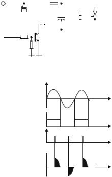
Figure 14.13 explains how the power transferred to the heater is controlled by controlling the delay between the moment when the ac voltage crosses zero and the moment when a pulse is generated by software to open the triac.
The actual output of the control circuit is a time delay: the shorter the delay, the longer time the triac stays in conduction, and the more power is transferred to the load.
14.4 Software Implementation of a PI Temperature Controller
The structure of the software for this application follows the general structure described in Chap. 9. The MAIN.ASM module includes a number of other ASM files, each associated with a particular function, or task. Here is the listing of the MAIN module:
TITLE PI CONTROLLER MAIN
INCLUDE 68HC11F1.DEF
INCLUDE AS11.MAC
INCLUDE MAP.ASM
180 |
14 |
PI Temperature Controller |
|
|
|
|
CODE |
|
|
|
|
VECTOR_RESET |
;RESET entry point |
|
|
RESET |
EQU |
* |
|
|
|
INCLUDE |
INIT.ASM |
;initializations |
|
MLOOP |
EQU |
* |
|
|
|
INCLUDE |
TIMER.ASM |
;software timers |
|
|
INCLUDE |
INPUT.ASM |
;digital&analog |
|
|
INCLUDE |
INTEGRAL.ASM |
|
|
|
INCLUDE |
CONTROL.ASM |
|
|
|
INCLUDE |
DISPLAY.ASM |
|
|
|
JMP |
MLOOP |
|
|
|
INCLUDE |
OUTPUT.ASM |
|
|
|
END |
|
|
The first two include files, 68HC11F1.DEF and AS11.MAC, are present unchanged in all HC11 applications described in this book. They contain the symbolic definitions of the I/O registers, and a set of useful macro definitions.
MAP.ASM defines the memory map, by specifying the beginning of the DATA and CODE segments, and also contains the definitions of all RAM variables used by the program. Although MAP.ASM contains application-specific code, a similar file must be present in all applications, along with INIT.ASM, which contains the initialization routines for all the resources used by the application. In this particular project, INIT.ASM has the following contents:
TITLE INITIALIZATION MODULE
CODE
SEI |
|
;disable all interrupts |
|
|
;during init sequence |
LDAA |
#$0A |
|
STAA |
HPRIO |
;TIC3 has the highest |
|
|
;priority |
LDAA |
#$05 |
;Enable CSPROG |
STAA |
CSCTL |
;for a 32k memory |
LDS |
#RAMEND |
;init stack pointer |
LDAA |
#$80 |
;init I/O ports |
STAA |
DDRA |
|
LDAA |
#$20 |
|
STAA |
DDRD |
|
JSR |
ITIMER |
;init TOC2 |
JSR |
IADC |
;init ADC |
JSR |
ITIC3 |
;init TIC3 |
JSR |
ISPI |
;init SPI |
JSR |
INITVAR |
;init variables |
CLI |
|
;enable interrupts |
END |
|
|
Note that the actual initialization sequences, associated with specific resources, are organized as subroutines (ITIMER, ISPI, IADC), and are located in the soft-ware modules dealing with the respective resources.

14.4 Software Implementation of a PI Temperature Controller |
181 |
The rest of the modules are included in an endless program loop. TIMER.ASM defines a set of software timers, as described in Chap. 9. INPUT.ASM reads the analog input lines AN0–AN3, connected to the temperature sensor and three external potentiometers, and updates the variables TS, TM, KP and TI. For scaling purposes, the 8-bit value read from AN2 is truncated to the four most significant bits, so that KP is limited to take values in the range [0–15]. Similarly, TI is reduced to take values in the range [0–63]. The digital input lines PA0–PA6 are read to update the variables SWSTATUS, which encodes the status of the rotary switch, and QSTART, a Boolean variable set to $FF when the START button is pressed, and cleared by pressing the STOP button. The subroutine CERR (Compute Error) is called here and updates the variable ERR – a 16-bit signed integer, defined as the difference (TS − TM).
The module INTEGRAL.ASM approximates the term:
Ti
1 × e(t)dt . Ti
0
Using the notation Ei = e(i × T0), then the integral can be approximated by the sum:
N |
|
|
|
N |
|
||
|
(T0 × Ei ) = T0 × |
|
Ei . |
(14.4) |
|||
i=1 |
|
|
|
i=1 |
|
||
If Ti = N × T0, then: |
|
|
|
|
|
|
|
|
|
|
Ti |
N |
Ei |
|
|
1 |
|
|
|
||||
× |
e(t)dt = |
i=1 |
(14.5) |
||||
|
|
|
|
. |
|||
|
Ti |
|
N |
||||
|
|
|
0 |
|
|
|
|
This means that the integral term in the expression (14.3) can be approximated by the average of the last N values of the variable ERR = TS − TM. The number N of samples considered for computing the integral is determined by the variable TI. T0 is a constant, equal to 100 ms, implemented by means of a software timer.
The values of the samples Ei are stored in a buffer IBUF. The size of IBUF must be dimensioned so that it can store the maximum value of samples, as indicated by the variable TI. Since TI can have one of 64 possible values, and the error ERR is a 16-bit integer, then IBUF must be128 bytes in length.
Two additional bytes are reserved for a pointer in IBUF, named XIBUF. IBUF is organized as a circular buffer. Each time the timer that defines T0 expires, the computed value of ERR is stored in the buffer at the location indicated by XIBUF, and then the pointer is incremented by 2. When the end of buffer is reached, the pointer is reloaded with the starting address of IBUF.
Only the last TI values in IBUF are used to compute the average. The result is stored in the variable INTEGRAL This is used by the module CONTROL.ASM, which computes VOUT = KP (ERR + INTEGRAL). VOUT is adjusted to be an 8-bit value in the range [0–255].
182 14 PI Temperature Controller
The computed value of VOUT is used in OUTPUT.ASM to determine the moment at wich to generate the pulse to open the triac that drives the heater. This is done in the interrupt service routine of TIC3. When an edge on IC3 (PA0) occurs, the TIC3 interrupt service routine prepares a value for TOC1, based on the value of VOUT, then enables the TOC1 interrupt.
To avoid time-consuming calculations in the interrupt service routine, VOUT is used as an offset in a table (TOCTAB) that contains for each possible value of VOUT, a 16-bit value that is added to the current TCNT and written to TOC1. These cause a TOC1 interrupt to be generated after a number of E cycles equal to the value extracted from TOCTAB.
The TOC1 interrupt service routine simply generates a pulse on PA7, then disables further TOC1 interrupts. A new interrupt will only be generated when an edge is sensed on IC3 and QSTART = $FF.
Here is what the interrupt service routines for TIC3 and TOC1 look like:
VECTOR_TIC3 |
|
|
LDAA |
TFLG1 |
;clear interrupt flag |
ORAA |
#$01 |
|
STAA |
TFLG1 |
|
LDX |
#TOCTAB |
|
LDD |
VOUT |
|
ABX |
|
;add VOUT as offset |
LDD |
0,X |
;get data from table |
ADDD |
TCNT |
|
STD |
TOC1 |
;prepare TOC1 interrupt |
LDAA |
#$80 |
;enable TOC1 interrupts |
ANDA |
QSTART |
;if QSTART=$FF |
BEQ |
TIC310 |
|
ORAA |
TMSK1 |
|
STAA |
TMSK1 |
|
RTI |
|
|
TIC310 LDAA |
TMSK1 |
;disable TOC1 interrupts |
ANDA |
#$7F |
;if QSTART=0 |
STAA |
TMSK1 |
|
RTI |
|
|
VECTOR_TOC1 |
|
|
LDAA |
TFLG1 |
|
ORAA |
#$80 |
;clear interrupt flag |
STAA |
TFLG1 |
|
LDAA |
#$80 |
;pulse on PA7 |
STAA |
PORTA |
|
NOP |
|
;wait a few microseconds |
NOP |
|
|
NOP |
|
|
NOP |
|
|
NOP |
|
|