3.1 OP Code Byte Addressing Modes

This section discusses addressing that is selected in the opcode byte, which is generally the first byte of the instruction. We have already introduced this idea in an ad hoc manner in Chapter 1 when we discussed implied, immediate, and direct addressing. Now we add page zero addressing and explain when each address mode should be used.

Some instructions do not involve any address from memory for an operand or a result. One way to avoid going to memory is to use only registers for all the operands. The DECinstruction decrements (subtracts one from) the value in an accumulator so that DECA and DECS are really the same operation, with the registers A and B serving as the addresses for the operand and result. Motorola considers DECA and DECB to be different instructions, whereas other manufacturers would call them the same instruction with a register address that indicates which register is used. Either case has some merits, but we will use Motorola's convention.

There is also an instruction

DEC 100

that recalls the word at location 100, decrements that word, and writes the result in location 100. That instruction uses direct addressing (as discussed in Chapter 1), whereas DECA does not use direct addressing. Because the instruction mnemonic for instructions such as DECA makes it clear which registers are being used, at least for simple instructions, Motorola calls this type of addressing inherent or implied. It is a zerolevel mode. For instance, CLRA clears accumulator A (puts its contents to zero) and uses inherent addressing, whereas

CLR 1000

clears the word at location 1000 and uses direct addressing. Several other instructions, such as SWI and BGND, which we are using as a halt instruction, have been included in the inherent category because the operation code byte of the instruction contains all of the addressing information necessary for the execution of the instruction.

We have used the immediate addressing mode in Chapter 1, where the value of the operand is part of the instruction,as in

LDAA #67

which puts the number 67 into accumulator A. We use the adjective "immediate" because when the instruction is being fetched from memory the program counter contains the address of the operand, and no further memory reads beyond those required for the instruction bytes are necessary to get its value.

You should use inherent addressing wherever it will shorten the program storage or speed up its execution, for example, by keeping the most frequently used data in registers as long as possible. Their use will involve only inherent addressing. Immediate addressing should be used to initialize registers with constants or provide constants for other instructions, such as ADDA.

For example,

LDAA <L,PCR

can load any word into A that can be reached by adding an 8-bit signed number to the program counter. (Recall that the PC is pointing to the next instruction just below the LDAA instruction when the effective address L is calculated.) The instruction

LDAA >L,PCR

can be used to access words that are farther away than -128 to + 127 locations from the address of the next instruction; it adds a 16-bit offset to the current value of the program counter to get the effective address. Although the machine coding of relative addressed instructions is the same as that of index addressed instructions, do not dwell too much on that similarity because the offset put in the machine code is determined differently.

Program counter relative indirect addressing can be used to access locations such as I/O ports as in

LDAA [L,PCR]

Assuming that L is 18 bytes below this instruction, the machine code is given by

where $A6 is the opcode byte for any LDAA index mode; the post byte $FB indicates indirect index addressing with 16-bit offset, but using the program counter as the "index register", and the last two bytes are added to the program counter. The indirect address ($12 in the example above) is in a location relative to the program. If the program is loaded into a different location, the offset $12 is still used to get the indirect address. Such use of relative and indirect relative addressing lets the program have one location and only one location where a value is stored, so that a downloaded file can insert the value in one place to run the program anywhere it is stored.

Branch and long branch instructions do not need the ",PCR" symbol in the instruction because they only use relative addressing with 16-bit relative offsets. However, the BSR L, having an 8-bit offset, doesn't have a corresponding long branch

to a subroutine whose address is in a "jump table," as discussed in a problem at the end of this chapter. Such jump tables make it possible to write parts of a long program in pieces called sections and compile and write each section in EEPROM at different times. Jumps to subroutine in a different section can be made to go through a jump table rather than going directly to the subroutine. Then when a section is rewritten and its subroutines appear in different places, only that section's jump table needs to be rewritten, not all the code that jumps to subroutines in that section. The jump table can be in EEPROM at the beginning of the section, or in RAM, to be loaded at run time.

Figure 3.11. A Stack Buffer for Two Stacks

The hardware stack, pointed to by SP, is useful for holding a subroutine's arguments and local variables. This will be discussed at the end of this section. However, because return addresses are saved on and restored from the hardware stack, we sometimes need a stack that is not the same as that hardware stack. For instance, we may push data in a subroutine, then return to the calling routine to pull the data. If we use the hardware stack, data pushed in the subroutine need to be pulled before the subroutine is exited, or that data will be pulled by the RTS instruction, rather than the subroutine's return address. A second stack can be implemented using an index register such as Y. If index register Y is also needed for other purposes in the program, this second stack pointer can be saved and restored to make it available only when the second stack is being accessed.

Figure 3.11 illustrates that a second auxiliary stack may use the same buffer as the hardware stack. The hardware stack pointer is initially loaded with the address of (one past) the high address of the buffer, while the second auxiliary stack pointer (Y) is loaded with (one below) the low end of the same stack buffer. The second stack pointer is initialized as: LDY #$B7F. Accumulator A can be pushed using STAA 1, +Y. A byte can be pulled into accumulator A using LDAA 1, Y- . A 16-bit word can be pushed and pulled in an obvious way. Observe that autoincrementing and autodecrementing are reversed compared to pushing and pulling on the hardware stack, because, as seen in Figure 3.11, their directions are reversed.

The advantage of having the second stack in the same buffer area as the hardware stack is that when one stack utilizes little of the buffer area, the other stack can use more of the buffer, and vice versa. You only have to allocate enough buffer storage for the worst-case sum of the stack sizes, whereas if each stack had a separate buffer, each buffer would have to be larger than the worst case size of its own stack.

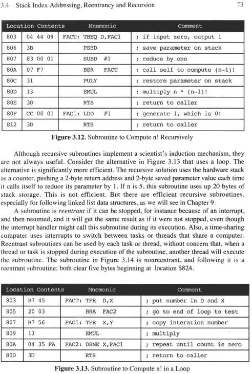
A recursive subroutine is one that calls itself. The procedure to calculate n factorial, denoted n!, is recursive; for any positive nonzero integer n, if n is one, n! is 1, otherwise n! is (n-1)! * n. The subroutine in Figure 3.12 calculates n!; upon entry, n is in accumulator D, and upon exit, n! is in accumulator D.

it is not clear whether the load is executed before the + or after the +. Note that if the latter is true, the + would have no effect on the instruction. Indeed, in the 6812, the + is carried out before the operation; in this case a load, so that

LDX 2,X+

is the same as

LDX 2,X -

For any load instruction involving the same index register for the location of the operand and the location of the result, the general rule is that postincrementing has no effect on the instruction. However, the fact that the postincrementing is carried out before the operation produces an unexpected result in the store counterpart of the load instruction just discussed. For example, with

STX 2,X+

suppose that X initially contains 373. After the instruction is executed, one will find that X becomes 375, and 375 has been stored in locations 373 and 374. We conclude this discussion by noting that predecrementing has none of these ambiguities. For example, if X initially contains 373 before the instruction

STX 2,-X

is executed, then 371 will be stored in locations 371 and 372.

There is often considerable confusion about LDX (direct), LDX #, and LEAX. Consider the following examples, assuming location $820 stores $1234.

LDX $820

will load $1234 into X. Direct addressing loads the data located at the instruction's address. However, immediate addressing loads part of the instruction into the register, as

LDX #$820

will load $820 into X. Sometimes, immediate addressing is used to load an address into memory so that pointer addressing (index addressing with zero offset) can access the data:

LDX #$820

LDX 0,X

will eventually load $1234 into X. Also, the LEAX instruction loads the effective address into an index register. When it is used with program counter relative addressing, it has the same effect as LDX # but is position independent.

LEAX $820,PCR

LDX 0,X

1 5. Write a shortest program segment beginning at $866 to call subroutine PRINT, at $852, with the address of the character string to be printed in index register X, first for a string stored at location $876 and then for one at $893. However, the calling program segment, the subroutines, and the strings may be in a single ROM that can be installed anywhere in memory. They are in locations fixed relatively with respect to each other (position independence). Show your machine code.

16.Write a shortest program segment to put square waves on each output port bit, at location 0 so bit i's square wave's period is 21 times the period of bit O's square wave.

17.Write a shortest program segment to add index register X to accumulator D, transferring the data on the auxiliary stack pointed to by Y, as shown in Figure 3.11.

18.Write a shortest program segment to exclusive-OR accumulator A into accumulator B, transferring the data on the auxiliary stack pointed to by Y, as shown in Figure 3.11.

19. The Fibbonacci number of 0, ^F(O) is 1, and ^F(l) is 1, otherwise ?(i) is ?(i - 1) + J(i - 2) for any positive integer i. Write a subroutine FIB that computes the

20. Write a subroutine POWER, with input signed number n in accumulator D and unsigned number m in index register X that computes nm leaving the result in accumulator D.

(a) Write a recursive subroutine, (b) Write a nonrecursive (loop) subroutine.

21. In Figure 3.16a, the instruction MOVW #$ 18bc, 1, SP writes to a local variable on the stack in the outer loop. Write an instruction to load this value into index register X, which is just inside the next inner loop, where the instruction LDAA 2, SP is. Write an instruction to load this value into index register X, which is just inside the innermost loop, where the instruction LDAA 6, SP is.

2 2. Assume that an overflow error can occur in an ADD instruction in the innermost loop in Figure 3.16a, just after the instruction LDAA 6, SP. The following instruction BVS L, after the ADD instruction, will branch to location L. Write an instruction at this location L to deallocate stacked local variables such that the stack pointer will be exactly where it was before the first instruction of this figure, LEAS -3,SP, was executed.

2 3. Write a shortest subroutine that compares two n-character null (0) terminated ASCII character strings, si and s2, which returns a one in accumulator B if the strings are the same and zero otherwise. Initially, X points to the first member of si (having the lowest address), Y points to the first member of s2, and n is in accumulator A.

24. Figure 3.21 shows a table where the first column is a 32-bit Social Security number; other columns contain such information as age; and each row, representing a person, is 8-bytes wide. Data for a row are stored in consecutive bytes. Write a shortest program segment to search this table for a particular social security number whose high 16 bits are in index register Y, whose low 16 bits are in accumulator D, and for which X contains the address of the first row minus 8. Assume that a matching Social Security number will be found. Return with X pointing to the beginning of its row.

An assembler is a program someone else has written that will help us write our own programs. We describe this program by how it handles a line of input data. The assembler is given a sequence of ASCII characters. (Table 4.1 is the table of ASCII characters.) The sequence of characters, from one carriage return to the next, is a line of assembly-language code or an assembly-language statement. For example,

would be stored as source code in memory for the assembler as:

The assembler outputs the machine code for each line of assembly-language code. For example, for line (1), the assembler would output the bytes $86 and $10, the opcode byte and immediate operand of (1), and their locations. The machine code output by the assembler for an assembly-language program is frequently called the object code. The assembler also outputs a listing of the program, which prints each assembly-language statement and the hexadecimal machine code that it generates. The assembler listing also indicates any errors that it can detect (assembly errors). This listing of errors is a great benefit, because the assembler program tells you exactly what is wrong, and you do not have to run the program to detect these errors one at a time as you do with more subtle bugs. If you input an assembly-language program to an assembler, the assembler will output the hexadecimal machine code, or object code, that you would have generated by hand. An assembler is a great tool to help you write your programs, and you will use it most of the time from now on.

In this chapter you will look at an example to see how an assembly-language program and assembler listing are organized. Then you will look at assembler directives, which provide the assembler with informationabout the data structure and the location of the instruction sequence but do not generate instructions for the computer in machine code. You will see some examples that show the power of these directives. The main discussion will focus on the standard Motorola assembler in their MCUez freeware.

At the end of this chapter, you should be prepared to write programs on the order of 100 assembly-languagelines. You should be able to use an assembler to translate any